1.2 Analysis of Distances

The results obtained in a PCA will allows us to get a visualization of the differences among the 51 cities, according to the net salaries of the chosen professions, as well as a visualization of the global association among such professions.

To get such visual displays, we utilize a geometric approximation that is fairly simple and intuitive. As a matter of fact, this type of approximation is the foundation of all component-based exploratory methods, which consists of regarding a data matrix from the dual point of view of rows and columns. Each perspective involves considering a cloud of points, one for the rows, and one for the variables.

1.2.1 Cloud of Row-Points

We can regard each row of the data table (each city) as one point with 12 coordinates. Each coordinate corresponding to each of the 12 professions.

If we had only recorded three professions, the values taken by each city would be located in a three dimensional space, defining a cloud of 51 city-points. We can generalize this idea to any number of professions. If we consider our 12 selected professions, then the cloud of points will be located in a 12-dimensional space.

In general, the rows of a data matrix will form a cloud of \(n\) points in a \(p\)-dimensional space (as many dimensions as active variables). We call this cloud the cloud of row-points or simply the cloud of individuals.

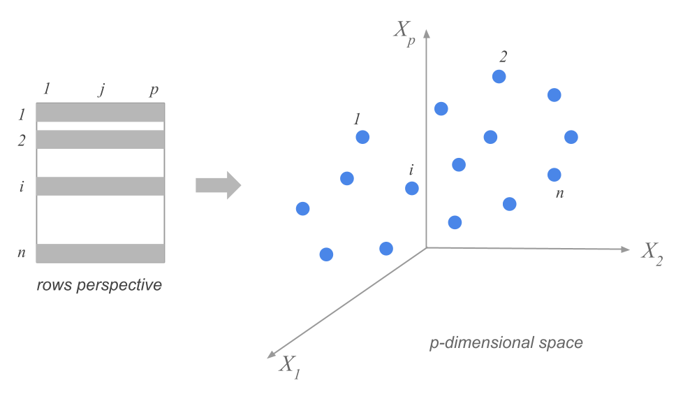
Figure 1.3: Cloud of n Row-points

In this cloud, two points that are close to each other will indicate two cities with similar values in each of the 12 professions. In contrast, two points that are further apart will indicate two cities with distinct salary levels.

To measure the notion of proximity between row-points (the cities) we need to define a measure of distance. The most intuitive distance measure is the euclidean distance between two points given by:

\[ d^2(i, i') = \sum_{j=1}^{p} (x_{ij} - x_{i'j})^2 \tag{1.1} \]

The main problem with visualizing the distance among the points, resides in the high dimensionality of the cloud of points (12 dimensions in our example) which makes it impossible to our human vision to visualize.

1.2.2 Cloud of Column-Points

In a similar way to the cloud of row-points, we can geometrically represent the \(p\) columns of the data matrix in an \(n\)-dimensional space (one dimension for each individual). The \(n\) coordinates of a column-point are given by the \(n\) values of the corresponding variable in the data table.

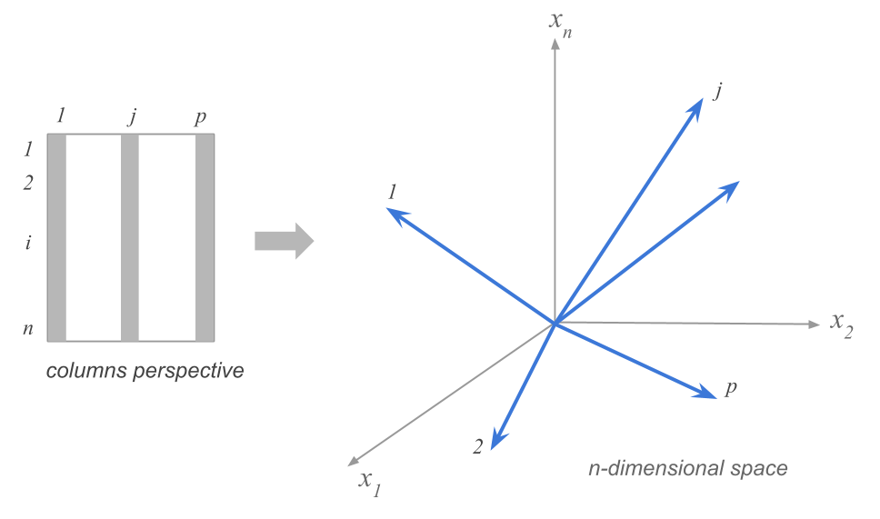
Figure 1.4: Cloud of p Column-points

The interesting part of this cloud of variable-points lies in the fact that it is a representation of the associations between the variables. Each of them measures an observed characteristic on the cities. Consequently, we can see which variables measure similar things among the cities. Analogous to the distance between cities, we need to define a distance between the variable-points that captures the intensity and the nature of the association between the variables.

Two variable-points that are close to each other, will indicate two variables that take related values in the entire set of cities: if we know the values of one variable, we can know the values of the other one.

A very common measure to quantify the association between variables is the linear correlation coefficient. If we used this coefficient as a distance, then the visualization of the variables becomes a visual display of the matrix of correlations among variables.