3.15 Conditional PCA
Often, after performing a PCA, we may find that its results are somewhat obvious, which, for inexperienced users, tends to produce a feeling a frustration about the capabilities of PCA. This has been the case for the data of international cities, where we know there is a size effect related with the first extracted factor, which makes the other factors relatively smaller. Another example in which this situation happens frequently is with socioeconomic data: it is not uncommon to see a first factor expressing the level of economic development. Similarly, with electoral data, we typically obtain a first factor that opposes “right” versus “left” (politically speaking). In these situations, we should go beyond the first factor; that is, we should eliminate (or control) the size effect and rerun PCA on the transformed data.
There are various ways to transform the data in order to control the size effect. One example has to do with the international cities in which, as you recall, we divided the salary of each profession by the mean city salary.
The point that we want to make is that Principal Components Analysis is a tool to explore a multivariate reality contained in a data set. The way in which we obtain the data to reflect the phenomena of interest, is a matter that pertains to the data scientist.
In other cases, PCA can reflect the variability that we are interested in studying. But such variability may be mixed with other uncontrolled significant effects, that interfer with our reading of the output. Which in turn can lead us to perplexity, and quitting the method. Only a very careful analysis on the sources of variability, allowing us to eliminate the undesired ones, will lead us to obtain satisfactory resutls.
3.15.1 PCA on Model Residuals
One way to eliminate the effects due to third-party variables consists of modeling the influence that such variables have on the analyzed data. With the model residuals, we can then apply PCA on them. Let \(\mathbf{X}\) be the data matrix of \(p\) continuous active variables, and let \(\mathbf{Z}\) be the matrix of \(q\) variables whose effect we wish to eliminate. Assuming a linear relationship between both sets of variables, we can then write:
\[\begin{align*} \mathbf{x_1} &= b_{11} \mathbf{z_1} + \dots + b_{1q} \mathbf{z_q} + \mathbf{e_1} \\ \vdots &= \vdots \\ \mathbf{x_p} &= b_{p1} \mathbf{z_1} + \dots + b_{pq} \mathbf{z_q} + \mathbf{e_p} \end{align*}\]
The matrix formed by the residuals \(\mathbf{e_j}\) (in the columns), denoted as \(\mathbf{E}\), reflect the variability of \(\mathbf{X}\) after having eliminated the linear part explaind by the variables of \(\mathbf{Z}\). Note that the adjusted model does not contain a constant term because we are assuming mean-centered variables.
The figure below illustrates the fitted result, and thus, the difference between the initial variables \(\mathbf{x_j}\) and the analyzed residual variables \(\mathbf{e_j}\)
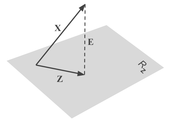
Figure 3.13: Multiple Regression of X-columns onto the space spanned by Z-columns
PCA of columns of \(\mathbf{E}\) implies analyzing the covariance matrix:
\[ \frac{1}{n} \mathbf{E^\mathsf{T} E} = \frac{1}{n} (\mathbf{X^\mathsf{T} X} - \mathbf{X^\mathsf{T} Z} (\mathbf{X^\mathsf{T} X})^{-1} \mathbf{Z^\mathsf{T} X}) = V(\mathbf{X} \mid \mathbf{Z}) \]
From the diagonal of \(V(\mathbf{X} \mid \mathbf{Z})\), we can calculate the partial correlations, and therefore, perform a normalized analysis on residuals. Is is also possible to mean-center and normalize the original variables \(\mathbf{x_j}\), and then perform PCA on the residuals, in order to give an importance to each variable based on the variability that is unexplained.
This PCA on a model’s residuals, is simple method that allows us to eliminate the effect of third-party variables, also known as instrumental variables, that relies on the goodness-of-fit of the explained model (Rao, 1964). In practice, other similar analysis are possible; in any case, one needs to estimate the model and then obtain the residuals to work with.
Notice that variables of matrix \(\mathbf{Z}\) may be reduced to just one variable, which can reflect for example, the time sequence, or the level of salary of individuals; it can also be one or more of the principal components found from a first analysis on the raw data. Likewise, the variable can be categorical, in which case it will define a partition of the individuals based on the category of each individual.
\[ \mathbf{Z} = \left[\begin{array}{cccc} 1 & 0 & \cdots & 0 \\ 1 & 0 & \cdots & 0 \\ 0 & 1 & \cdots & 0 \\ \vdots & \vdots & \ddots & \vdots \\ 0 & 0 & \cdots & 1 \\ \end{array}\right] \]
In this case, the analyzed residuals express the difference between the value taken by each individual in a given variable, and the mean value of such variable, among the group of individuals to which it belongs, based on the partition defined by \(\mathbf{Z}\).
\[ \hat{x}_{i_k j} = \frac{1}{n_k} \sum_{\ell_k = 1}^{n_k} x_{\ell_k s} \qquad e_{ij} = x_{ij} - \hat{x}_{ij} \tag{3.12} \]
where \(i_k\) indicates an individual belonging to the \(k\)-th group of individuals.
3.15.2 Analysis of Local Variation
PCA of a model residuals is based on how well the model translates the effect of variables in \(\mathbf{Z}\) on the data we are analyzing. In addition, we need to keep in mind the underlying assumptions of the model, which may not be easy to fulfill in practice. Under these conditions, a non-parametric alternative, especially interesting when dealing with large data sets, consists of performing what is called a local PCA. The idea of this analysis is to construct an undirected graph among individuals, in such a way that it reflects the effect we are interested in eliminating.
For example, if we want to eliminate the effect of the perceived income, the graph will be built by connecting the individuals that have an equal perceived income, or an income that differs at most by a certain quantity below a predefined threshold. If we want to eliminate the effect “North/South” in a socioeconomic study of geographical units, then the graph will express a relation of contiguity between the geographic units under analysis. If we wish to eliminate the effect due to gender, the graph will be formed by connecting all the men among them, and all the women among them.
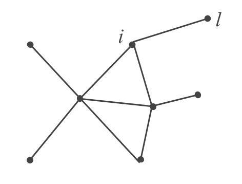
Figure 3.14: Example of a graph (the nodes are individuals and the edges connect similar individuals based on the variables whose effect we want to eliminate)
The most natural way to define a model between the variables \(\mathbf{x_j}\) eliminating the effect of variables \(\mathbf{z_j}\), involves using the local regression from the neighbors of each individual \(i\) in the graph (Benali et al, 1990). Let \(n_i\) be the number of neighbors of individual \(i\), and let \(\mathcal{l}_i\) be the set formed by all of them.
\[ \hat{x}_{ij} = \frac{1}{n_i} \sum_{v_i \in l_i}^{ni} x_{v_i j} \qquad e_{ij} = x_{ij} - \hat{x}_{ij} \]
where \(v_i\) identifies the neighbors of individual \(i\). Notice that the above formula allows us to tune the similarity of an individual \(i\) in a much better way than the one provided in formula (3.12) where an individual is absorbed by the group to which it belongs.
Regardless of the utilized method for modeling the variables \(\mathbf{X}\), we always decompose the covariance matrix into two terms: one term explains the variables \(\mathbf{Z}\), whose effect we want to eliminate; the other term expresses the remaining or residual variability. The conditional analysis involves analyzing this latter term
\[ \mathbf{V} = \mathbf{V_{\text{explained}}} + \mathbf{V_{\text{residual}}} \]
We should mention that an equivalent decomposition can be obtained by working with the differences between adjacent nodes in the graph.
The usefulness of this conditioning method derives from the generality of the graph. Such graph does not depend on any model, and can be defined ad-hoc based on the analyzed problem. For example, we can study the different sources of variability in ternary tables (one table observed in several occasions) by working on several graphs. One possible analysis implies connecting all individuals of the same occasion. Then the local PCA becomes an analysis of the variability among individuals, controling the “trend” or evolution between different occasions. Likewise, we can join all homologous individuals between different occasions. In this case, the local PCA reflects the oppositions of the same individual through different occasions, that is, the evolution between occasions, without taking into account the within-individuals variability. On these basic graphs, we could introduce other conditions, for example, that of individuals having a certain size above a given threshold, etc.