2.2 Projections of Variables
Just like row-points can be represented on a low-dimensional factorial space that preserves as much as possible the original distances, we can do the same with the column-points (i.e. the variables).
Mathematically, working with the column-points implies diagonalizing the cross-product matrix \(\mathbf{X X^\mathsf{T}}\).
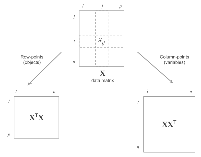
Figure 2.6: Matrices to be diagonalized depending on the type of points
Analogously to the row-points, we can obtain the decomposition of the inertia depending on the directions defined by the eigenvalues of the matrix \(\mathbf{X X^\mathsf{T}}\). The projected inertia on each direction is equal to its associated eigenvalue.
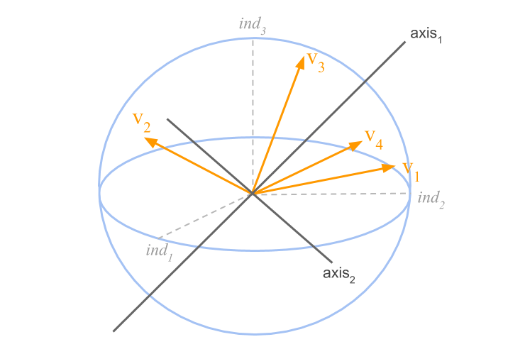
Figure 2.7: Cloud of variables and factorial axes in the space of individuals
The line of maximum inertia is given by the eigenvector \(\mathbf{v}\) (defining the direction \(F_1\)), associated to the largest eigenvalue. The plane of maximum inertia is formed by adding the line that defines the direction \(F_2\). This second direction corresponds to the eigenvector associated to the second largest eigenvalue, and so on.
The representation of the variables on an axis is obtained by projecting the variable-points onto a unit vector \(\mathbf{v}\) that defines the direction of the axis.
Let \(\varphi_{j \alpha}\) be the coordinate of the \(j\) variable on the axis \(\alpha\)
\[ \varphi_{j \alpha} = \sum_{i=1}^{n} \frac{x_{ij} - \bar{x}_j}{s_j} \hspace{1mm} v_{i \alpha} \tag{2.8} \]
where \(\bar{x}_j\) is the mean of the \(j\)-th variable.
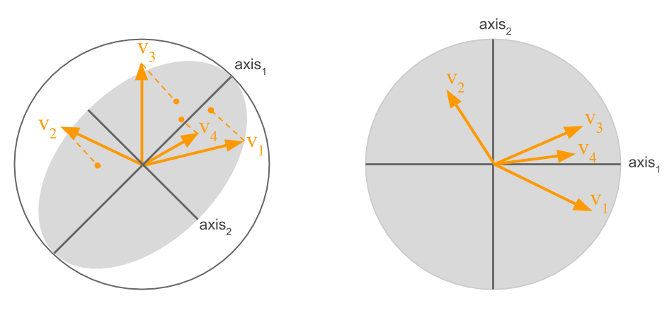
Figure 2.8: Projection of the variables on the first factorial plane
The inertia on an axis is given by the sum of the inertias of each variable-point projected onto the axis. In PCA there is not an explicit weight for the variable-points. However, each variable can play a role more or less important by changing the unit of measurement, which in turn will increase (or decrease) its variance in a non-normalized PCA.
\[ \sum_{j=1}^{p} \varphi^{2}_{j \alpha} = \lambda_{\alpha} \tag{2.9} \]
Notice that the inertia of the variable-points that are projected onto an axis is the same as the inertia of the row-points projected on the axis of same rank.
Among the factorial axes of both clouds of points, the factorial axes in one space are related to the factorial axes in the other space. These relationships allow us to obtain the directions of one space taking into account the directions of the other space. Such relationships are known as transition relationships.
By using the transition relationships, we just need to perform a PCA on one of the spaces (e.g. the rows), and then use these results to derive the results of the other space (e.g. the columns), without having to diagonalize two different cross-products.
In general, we perform the analysis on the cross-product with the smaller dimensions. Usually, this involves working with the matrix \(\mathbf{X^\mathsf{T} X}\), assuming that the data matrix has more rows than columns: \(n > p\). In this scenario, we obtain the projection of the row-points given in equation (2.1). The projection of the variables is then calculated from the directions \(\mathbf{u}\), which define the factorial axes of the cloud of row-points.
\[ \varphi_{j \alpha} = \sqrt{\lambda_{\alpha}} \hspace{1mm} u_{j \alpha} \tag{2.10} \]
The above formula allows us to interpret the simultaneous representation of both the cities and the professions.
In our working example, the results about the variables are displayed in table 2.3
| coord1 | coord2 | coord3 | cor1 | cor2 | cor3 | |
|---|---|---|---|---|---|---|
| teacher | 0.94 | -0.04 | -0.21 | 0.94 | -0.04 | -0.21 |
| bus_driver | 0.96 | -0.13 | -0.15 | 0.96 | -0.13 | -0.15 |
| mechanic | 0.92 | -0.27 | 0.19 | 0.92 | -0.27 | 0.19 |
| construction_worker | 0.90 | -0.37 | 0.11 | 0.90 | -0.37 | 0.11 |
| metalworker | 0.95 | -0.24 | -0.02 | 0.95 | -0.24 | -0.02 |
| cook_chef | 0.87 | 0.24 | 0.40 | 0.87 | 0.24 | 0.40 |
| factory_manager | 0.84 | 0.49 | -0.01 | 0.84 | 0.49 | -0.01 |
| engineer | 0.90 | 0.27 | -0.03 | 0.90 | 0.27 | -0.03 |
| bank_clerk | 0.88 | 0.38 | -0.13 | 0.88 | 0.38 | -0.13 |
| executive_secretary | 0.97 | 0.00 | -0.10 | 0.97 | 0.00 | -0.10 |
| salesperson | 0.96 | 0.01 | 0.08 | 0.96 | 0.01 | 0.08 |
| textile_worker | 0.94 | -0.25 | -0.10 | 0.94 | -0.25 | -0.10 |
The coordinates of all the variables in the first axis have the same sign, which indicates that the cloud of points is not centered.
Notice also that, in the case of normalized analysis, the coordinate coincides with the correlation of a variable and the principal component (projection of the points onto the factorial axis of same rank):
\[ \varphi_{j \alpha} = cor(\mathbf{x_j}, \boldsymbol{\psi_{\alpha}}) \tag{2.11} \]
This formula plays an important role in the interpretation of the results because it connects the representation of the row-points with the representation of the column-points.
A high correlation implies that the configuration of the individuals on a factorial axis resembles the positions of the individuals on that variable (a unit correlation would indicate that the principal component is a linear function of the variable). A correlation close to zero indicates that there is no linear association between the principal component and the variable.
2.2.1 Size Effect
As we’ve described it, the first principal component arises from the high correlation that exists among all the variables, which geometrically forms a very homogeneous array of vectors. This first component approximately corresponds to the bisector of this array of vectors, and will therefore be highly correlated to the original variables.
How can we interpret this phenomenon? Broadly speaking, for any city, if a salary is high in a given profession, then this is also true for the set of professions in that city. This general phenomenon is actually present in the entire data table as a structural pattern, which generates the first factor. And it is for this reason that we call the first component the size factor or size effect.
| exe | sal | bus | met | tea | tex | mec | eng | con | ban | coo | dep | |
|---|---|---|---|---|---|---|---|---|---|---|---|---|
| exe | ||||||||||||
| sal | 0.94 | |||||||||||
| bus | 0.93 | 0.89 | ||||||||||
| met | 0.92 | 0.88 | 0.94 | |||||||||
| tea | 0.92 | 0.88 | 0.96 | 0.91 | ||||||||
| tex | 0.93 | 0.89 | 0.92 | 0.94 | 0.88 | |||||||
| mec | 0.88 | 0.89 | 0.89 | 0.93 | 0.84 | 0.89 | ||||||
| eng | 0.87 | 0.85 | 0.82 | 0.80 | 0.81 | 0.81 | 0.74 | |||||
| con | 0.86 | 0.86 | 0.88 | 0.93 | 0.83 | 0.92 | 0.95 | 0.70 | ||||
| ban | 0.87 | 0.85 | 0.80 | 0.72 | 0.82 | 0.73 | 0.70 | 0.85 | 0.64 | |||
| coo | 0.80 | 0.85 | 0.76 | 0.76 | 0.75 | 0.71 | 0.80 | 0.82 | 0.72 | 0.79 | ||
| dep | 0.80 | 0.79 | 0.74 | 0.69 | 0.78 | 0.65 | 0.64 | 0.87 | 0.59 | 0.89 | 0.82 |
Having a first principal component that captures the size effect is a common phenomenon in PCA. A distinctive trait is that the matrix of correlations between the variables can be arranged based on the correlations with the first principal component. As we can tell from table 2.4, there are high correlations close to the diagonal, and then they decrease as one moves away from this diagonal.
Interpretation of the Axes
To better interpret a factorial axis we should take into account the variables that have a relative high correlation with the axis.
We have seen that the first axis is interpreted as a factor of size: differentiating cities according to their overall salary levels. The subsequent principal components comprise factors that are orthogonal to the first one.
The first principal component (projection of the cities onto the first direction of the cloud of row-points) provides an ordination of the cities depending on their salary levels. This first component opposes Swiss cities (Zurich and Geneva) and Tokyo to cities like Mumbai, Manila and Nairobi.
The second factorial axis, showing lower correlations with the original variables, opposes the professions factory_manager, engineer, bank_clerk, and cook_chef to textile_worker, construction_worker, mechanic, and metalworker. In other words, the second axis has to do with the fact that, independently from the salaries of a city, certain professions have a higher salaries than others.
The projection onto the second axis allows to distinguish cities with similar overall level of salaries: certain cities tend to value the managerial jobs, whereas other cities tend to value the professions less socially appreciated.
2.2.2 Tools for Interpreting Components
Cosine Squares
In a similar fashion to the analysis of the individuals (i.e. the cities), we can also define a set of coefficients, squared cosines, and contributions, that will help us in the interpretation of results in the analysis of the variables.
The squared cosines are defined as the quotient between the projected squared distance on an axis and the squared distance to the origin.
We know that the squared distance of a variable to the origin is equal to its variance:
\[ COS^2(j, \alpha) = \frac{\varphi^{2}_{j \alpha}}{var(j)} \tag{2.12} \]
The sum of the squared cosines over all the axes is always equal to one:
\[ \sum_{\alpha = 1}^{p} COS^2(j, \alpha) = 1 \tag{2.13} \]
In the normalized PCA, the variances are equal to one; thus the squared cosines will be squared of the coordinates of the variables:
\[ COS^2(j, \alpha) = \varphi_{j \alpha}^{2} \qquad \text{in normalized PCA} \]
In general, we have that:
\[ COS^2(j, \alpha) = CORR^2(\text{variable}, \text{factor}) \]
Contributions
The contribution of each variable to the inertia of an axis is the part of the inertia accounted for the variable. The inertia of an axis (see eq (2.9)) is expressed as:
\[ \lambda_{\alpha} = \sum_{j=1}^{p} \varphi_{j \alpha}^{2} \]
The contribution of a variable to the construction of an axis is:
\[ CTR(j, \alpha) = \frac{\varphi_{j \alpha}^{2}}{\lambda_{\alpha}} = \frac{(\sqrt{\lambda_{\alpha}} \hspace{1mm} u_{j \alpha})^2}{\lambda_{\alpha}} = u_{j \alpha}^{2} \tag{2.14} \]
where \(u_{j \alpha}^{2}\) is the coordinate of the former unit axis associated to the variable \(j\), projected on the axis \(\alpha\).
We have the following result:
\[ CTR(j, \alpha) = (\text{former unit axis})^2 \]
To find how much a variable contributes to the construction of an axis, it suffices to square each component of the vector \(\mathbf{u}\). These contributions indicate which variables are responsible for the construction of each axis. The sum of all the contributions to an axis is equal to 1 (or 100 in percentage).
\[ \sum_{j=1}^{p} CTR(j, \alpha) = 100 \tag{2.15} \]
The elements of \(\mathbf{u}\) define the linear combinations of the original variables, orthogonal among each other, and of maximum variance (i.e. the principal components). For example, the linear combination of the first component is:
\[ \boldsymbol{\psi_1} = 0.30 \texttt{ teacher} + 0.30 \texttt{ bus_driver} + 0.29 \texttt{ mechanic} \\ + 0.28 \texttt{ construction_worker} + 0.30 \texttt{ metalworker} + 0.27 \texttt{ cook_chef} + \\ +0.26 \texttt{ factory_manager} + 0.28 \texttt{ engineer} + 0.28 \texttt{ bank_clerk} + \\ + 0.31 \texttt{ executive_secretary} + 0.30 \texttt{ salesperson} + 0.29 \texttt{ textile_worker} \]
where each variable has been mean-centered and standardized (because we have performed a normalized PCA).
The first component is therefore defined by a set of coefficients, very similar to each other. In this particular case, the first component is not that different from the average of all the profession salaries.
The set of components \(u_{j \alpha}\) also define the projection of the former unit axes onto the new factorial axes.