1.1 Data and Goals

Behind a Principal Component Analysis, the analyst has to deal with several continuous variables measured on a number of individuals. The goal is to learn and gain insight about the available data. For instance, a common application of PCA has to do with building an economic index that measures the economic capacity of a group of individuals; PCA can also be used to obtain an optimal subset of points in order to control the polution in a certain geographic region; or to segment a population in terms of preference evaluations given to a group of similar products in a certain market.

Often, PCA can be used as an intermediate step in which its outputs will be part of a subsequent analysis such as regression, clustering, or classification. Likewise, it is also possible to employ PCA as a data compression methodology.

The starting point is a data set in which a number of continuous variables have been measured on a group of individuals. Sometimes, qualitative variables may also be present in the data.

The typical convention is to have a data set in a tabular format like in a spreadsheet (e.g. rows and columns). Virtually in all cases, the dimensions of the table will make it impossible to observe, by simple inspection, which individuals are similar, or which variables are measuring similar features among the individuals. In other words, the association structure of the variables, as well as the configuration of the similarities among individuals, remains hidden.

Let’s consider a simple example that will allows us to settle the various concepts underlying a Principal Component Analysis. The goal is to compare a given number of cities according to the mean salary-level of a dozen of occupations. The aim is to contrast the coherence of the description against our global economic knowledge.

The data set pertains to the year 1994, and it consists of 51 cities around the world, on which 40 economic variables have been measured. The cities are grouped in 10 regions around the world.

Num	Variable	Description
1	city	Name of the city
2	region	Region of the world
3	price_index_no_rent	Index of prices without renting cost
4	price_index_with_rent	Index of prices with renting cost
5	gross_salaries	Index of gross salaries
6	net_salaries	Index of net salaries
7	work_hours_year	Yearly worked hours
8	paid_vacations_year	Yearly paid vacations
9	gross_buying_power	Gross buying power
10	net_buying_power	Net buying power
11	bread_kg_work_time	Worked time to buy 1 kg of bread
12	burger_work_time	Worked time to buy a burger
13	food_expenses	Food expenses
14	shopping_basket	Cost of shopping basket (groceries)
15	women_apparel	Cost of women apparel
16	men_apparel	Cost of men apparel
17	bed4_apt_furnished	Cost of 4-bedroom appt. furnished
18	bed3_apt_unfurnished	Cost of 3-bedroom appt. unfurnished
19	rent_cost	Cost of house rent
20	home_appliances	Cost of home appliances
21	public_transportation	Public transportation (bus, train, metro)
22	taxi	Cost of taxi
23	car	Cost of car
24	restaurant	Cost of restaurant
25	hotel_night	Cost of one hotel night
26	various_services	Cost of various services
27	tax_pct_gross_salary	Taxes as percentage of gross salary
28	net_hourly_salary	Net hourly salary
29	teacher	Salary of School teacher
30	bus_driver	Salary of Bus driver
31	mechanic	Salary of Car mechanic
32	construction_worker	Salary of Construction worker
33	metalworker	Salary of Metalworker
34	cook_chef	Salary of Cook chef
35	departmental_head	Salary of Departmental head
36	engineer	Salary of Engineer
37	bank_clerk	Salary of Bank clerk (cashier)
38	executive_secretary	Salary of Executive secretary
39	salesperson	Salary of Salesperson (sales associate)
40	textile_worker	Salary of Textile worker

In the data table, the rows correspond to the individuals, which in this case have to do with the cities. In turn, the columns correspond to the variables which have to do with the characteristics measured on the cities.

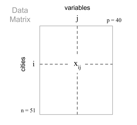
Figure 1.1: Standard format of a data matrix

Before performing the actual PCA, we should always carry out an exploratory analysis. This analysis refers to computing summary statistics such as maximum values, miminum values, range, measures of center, measures of spread, looking at the distribution of the variables (e.g. boxplots, histograms), etc. This preliminary analysis could help us identify outliers, errors, or other major anomalie in the data that can disturb that analysis and make the results worthless.

1.1.1 Active Variables

The data set of cities and economic variables is relatively small. However, the information contained in this data is very rich. There is a wide number of variables, which is typical of this type of applications. The variables can be grouped by topics. For instance, there is a series of variables that correspond to expenses (in clothes, home rent, vehicles, utilities, etc.). that reflect the cost of living in each city. Other variables involve information about the salary, broken down into 12 professions. Likewise, other variables convey information about the quality of life, such as taxes, payed vacations, work days, and so on.

To compare the cities, we can certainly take all the (continuous) variables and perform a Principal Component Analysis. Notice that this task will lead us to compare the cities in terms of prices, salaries, taxes, work-hours necessary to buy a hamburger, etc. The observed differences among cities are difficult to interpret; they can have multiple causes, and have values of very different nature.

Instead of selecting all the available variables, it is preferable to select a group of variables, more homogeneous according to a certain topic, and more aligned with the goals of the analysis. In this sense, what we call a topic is a group of variables which defines a certain standpoint, chosen by the analyst, to compare the cities. In this way, the interpretation of the proximities among cities will be easier.

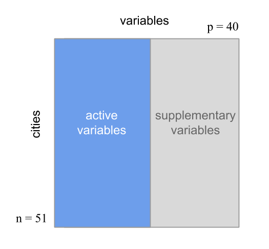
Figure 1.2: Selection of active variables and supplementary variables

The chosen variables, called active variables, comprise the unique elements that will be used to compare the cities among them. The rest of the variables that are not active are called supplementary variables. This does not mean that the information of the supplementary variables will not be used. We will use the supplementary variables as additional information that may help us to explain the observed (dis)similarities among the cities.

In our example, we will take as active variables the net income, measured in dollars, for the 12 selected professions. Two cities will be close to each other if the incomes of these 12 professions are very similar, independently of any other variables that may make them different (e.g. size, prices, altitude, etc.). In the following list we provide the 12 available professions:

• Teacher
• Bus driver
• Car Mechanic
• Construction worker
• Metalworker
• Cook chef
• Factory manager
• Engineer
• Bank clerk
• Executive secretary
• Salesperson
• Textile worker

The rest of the variables will be considered supplementary and they will be employed during the interpretation of the results.