3.4 Analysis of Table of Ranks
In PCA, it is assumed that the variables are measured on a continuous scale. When applying a normalized PCA, the results will depend on the matrix of correlations between variables. Such results can be affected by the presence of outliers or atypical observations.
One approach to make the results independent from the scale of measurement and monotone transformations, consists of working with the ranks of the variables and not with the actual observed values.
To do that, we substitute each value by its rank in increasing order, depending on the considered variable. By doing this, the active table becomes a table of ranks, and consequently, the PCA is performed on a correlation matrix of ranks. This is a remarkable feature of PCA: it is a general methodology that can be applied on any correlation matrix defined by the analyst.
One interesting transformation involves working with the Spearman’s correlation coefficients. This coefficient measures the monotone dependency between the rank values of two variables according to the following formula:
\[ r_s (j, j') = 1 - \frac{6 \sum_{i}^{n} (x_{ij} - x_{ij'})^2}{n (n^2 - 1)} \tag{3.4} \]
where the quantities \(x_{ij}\) represent the rank of the individual \(i\) of the \(j\) variable. The advantage of the Spearman’s correlation coefficient is that it coincides with the Pearson’s coeffcient (usual correlation coefficient) when applied to a matrix of ranks.
In the case of the international cities, the Spearman’s correlations are given in table 3.6 (compare these with table 2.6).
| tea2 | bus2 | mec2 | con2 | met2 | coo2 | dep2 | eng2 | ban2 | exe2 | sal2 | tex2 | |
|---|---|---|---|---|---|---|---|---|---|---|---|---|
| tea2 | 1.00 | |||||||||||
| bus2 | 0.22 | 1.00 | ||||||||||
| mec2 | -0.24 | 0.03 | 1.00 | |||||||||
| con2 | 0.27 | 0.28 | 0.31 | 1.00 | ||||||||
| met2 | 0.16 | 0.03 | 0.19 | 0.11 | 1.00 | |||||||
| coo2 | -0.24 | -0.21 | -0.20 | -0.43 | -0.33 | 1.00 | ||||||
| dep2 | -0.10 | -0.14 | -0.42 | -0.61 | 0.03 | 0.24 | 1.00 | |||||
| eng2 | -0.15 | -0.33 | -0.38 | -0.68 | 0.02 | 0.28 | 0.49 | 1.00 | ||||
| ban2 | 0.03 | 0.01 | -0.46 | -0.37 | -0.37 | 0.24 | 0.46 | 0.26 | 1.00 | |||
| exe2 | -0.22 | -0.28 | -0.59 | -0.60 | -0.36 | 0.19 | 0.41 | 0.49 | 0.37 | 1.00 | ||
| sal2 | 0.02 | -0.07 | -0.07 | -0.13 | -0.17 | -0.04 | 0.01 | 0.09 | -0.05 | 0.13 | 1.00 | |
| tex2 | 0.16 | 0.27 | -0.04 | 0.41 | 0.02 | -0.42 | -0.32 | -0.25 | -0.30 | -0.04 | 0.06 | 1 |
We apply a PCA on the matrix of Spearman’s correlations. The eigenvalues are depicted in table 3.7 which can be compared to those of table 2.7.
| num | eigenvalue | percentage | cumulative |
|---|---|---|---|
| 1 | 3.8758 | 32.30 | 32.30 |
| 2 | 1.6301 | 13.58 | 45.88 |
| 3 | 1.3199 | 11.00 | 56.88 |
| 4 | 1.2365 | 10.30 | 67.19 |
| 5 | 0.9125 | 7.60 | 74.79 |
| 6 | 0.8049 | 6.71 | 81.50 |
| 7 | 0.6575 | 5.48 | 86.98 |
| 8 | 0.4481 | 3.73 | 90.71 |
| 9 | 0.3752 | 3.13 | 93.84 |
| 10 | 0.3372 | 2.81 | 96.65 |
| 11 | 0.2662 | 2.22 | 98.87 |
| 12 | 0.1360 | 1.13 | 100.00 |
Likewise, table 3.8 displays the results obtained for the ranks of the active variables.
| coord1 | coord2 | coord3 | cor1 | cor2 | cor3 | |
|---|---|---|---|---|---|---|
| teacher2 | -0.27 | 0.59 | 0.37 | -0.27 | 0.59 | 0.37 |
| bus_driver2 | -0.39 | 0.45 | 0.00 | -0.39 | 0.45 | 0.00 |
| mechanic2 | -0.58 | -0.65 | -0.11 | -0.58 | -0.65 | -0.11 |
| construction_worker2 | -0.85 | 0.16 | -0.14 | -0.85 | 0.16 | -0.14 |
| metalworker2 | -0.32 | -0.22 | 0.84 | -0.32 | -0.22 | 0.84 |
| cook_chef2 | 0.55 | -0.30 | -0.30 | 0.55 | -0.30 | -0.30 |
| factory_manager2 | 0.71 | 0.07 | 0.38 | 0.71 | 0.07 | 0.38 |
| engineer2 | 0.73 | -0.08 | 0.31 | 0.73 | -0.08 | 0.31 |
| bank_clerk2 | 0.60 | 0.35 | -0.09 | 0.60 | 0.35 | -0.09 |
| executive_secretary2 | 0.75 | 0.27 | -0.16 | 0.75 | 0.27 | -0.16 |
| salesperson2 | 0.11 | 0.15 | -0.26 | 0.11 | 0.15 | -0.26 |
| textile_worker2 | -0.46 | 0.51 | -0.11 | -0.46 | 0.51 | -0.11 |
The cloud of points is depicted in figure 3.2. The configuration of this cloud is similar to the initial cloud displayed in figure 2.9. The similarity of the results obtained with the table of ratios confirms the good quality of the performed analysis. Also, this similarity shows that the essential information is contained in the rank of the values, and not so much in the observed values.
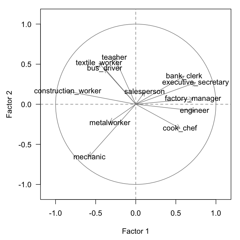
Figure 3.2: Circle of correlations on the first factorial plane of the second analysis
The fact that the cloud of points in figure 3.2 is similar to the graph 2.9, indicates that the visual displays do not depend on: the units of measurement, monotone transformations, or possible existance of outliers. Hence, we can say that the observed configurations are robusts.
In the absence of robust configurations, we can suggest positioning the elements of the original table as supplementary elements in the analysis of ranks, in order to detect whether there are sensible elements.
Sometimes it is convenient to work with variables that have distributions close to a normal distribution. In this case, each variables con be handled as having a normal distribution with expected value equal to the observation of rank \(k\), instead of working directly with the ranks (Lebart et al, 1977).