3.8 PCA and Clustering

The graphics obtained from Principal Components Analysis provide a quick way to get a “photo” of the multivariate phenomenon under study. These graphical displays offer an excellent visual approximation to the systematic information contained in data.

Having said that, such visual approximations will be, in general, partial approximations. This is because those low dimensional representations are given by scatterplots in which only two dimensions are taken into account. Unless the information in data is truly contained in two or three dimensions, most graphics will give us a limited view of the multivariate phenomenon.

Together with these graphical low dimensional representations, we can also use clustering methods as a complementary analytical tasks to enrich the output of a PCA. In clustering, we look for groups of individuals having similar characteristics. An individual is characterized by its membership to a certain cluster. In turn, the average characteristics of a group serve us to characterize all individuals in the corresponding cluster.

We can take the output of a clustering method, that is, take the clustering memberships of individuals, and use that information in a PCA plot. The location of the individuals on the first factorial plane, taking into consideration their clustering assignment, gives an excellent opportunity to “see in depth” the information contained in data. In other words, with the formed clusters, we can see beyond the two axes of a scatterplot, and gain deeper insight into the factorial displays.

3.8.1 Real Groups or Instrumental Groups?

Given a clustering partition, an important question to be asked is to what extent the obtained groups reflect “real” groups, or are the groups simply an algorithmic artifact? Do we have data that has discontinuous populations, or do we just have a continuous reality?

In general, most clustering partitions tend to reflect intermediate situations. Sometimes we may find clusters that are more or less “natural”, but there will also be times in which the clusters are more “artificial”. Intermediate situations have regions (set of individuals) of high density embedded within layers of individuals with low density. Even in such intermediate cases, the obtained clustering partition is still useful. While we cannot say that clusters are “real” groups differentiated from one another, the formed groups makes it easier to understand the data. In this sense, clustering acts in a similar fashion as when we make bins or intervals from a continuous variable. Simply put, clustering plays the role of a multivariate encoding. This is why we talk about instrumental groups.

In the example of international cities, we obtain the following dendrogram from a hierarchical agglomerative clustering on the data of ratios.

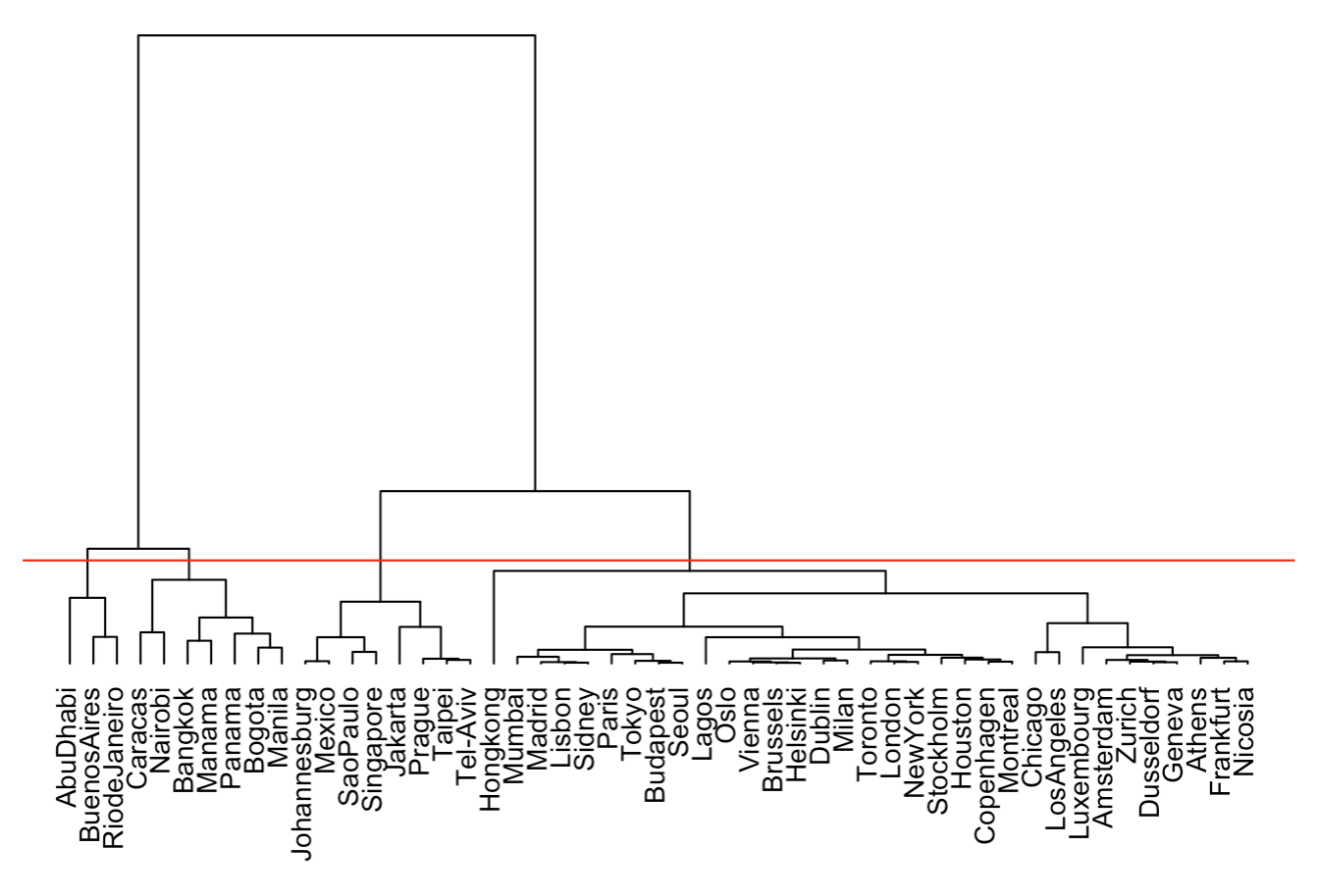
Figure 3.5: Clustering Dendrogram

Looking at the dendrogram, we can identify the existence of several groups of cities.

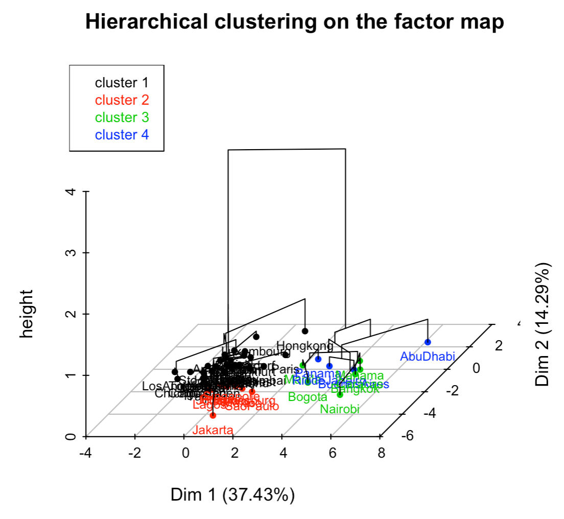
The obtained partitions are projected on the factorial plane, that is, the centroids of each clustered are projected together with the cities, colored by group, as depicted in the following figure:

On one hand, the 10 cities that are grouped in the first cluster are highly homogeneous, and distinct from other cities. The cutting line (red horizontal line) isolates well this group, while producing at the same time other three different clusters.

Ths cluster of 10 cities involves cities with a large salary inequality, with high salaries for those managerial/head-type of professions. Opposed to this group, there is a considerably large cluster characterized for having elevated taxes as well as social contributions, and for having better well payed professions that are generally considered to be “lower class”.

Separated from the large cluster, there are two more groups, distinguished on the second factorial axis. One of them is formed by cities with high salaries for manual-labor professions. The other group is formed by those cities with high salaries for professions that depend on the Public Service.

The obtained partitions are projected on the factorial plane, that is, the centroids of each clustered are projected together with the cities, colored by group, as depicted in the following figure:

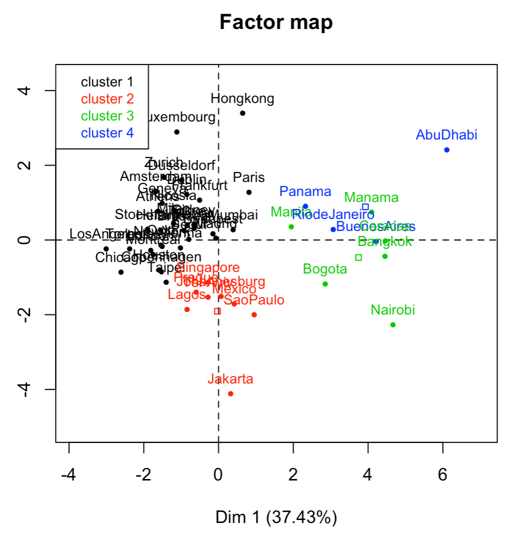
Figure 3.6: Clustering of cities in 4 groups

3.8.2 Representants of Groups

For every cluster, we can calculate its corresponding centroid (i.e. average individual). We can also determine the individual that is the closest to the centroid, called the representant. Likewise, we can also look for the second best representant, the third best representant, etc.

If we establish the radius of circle (or sphere) around the centroid of a given cluster, we can capture the representants of the cluster. For a small radius, we may get just one representant. As we increase the value of the radius, more representants will be captured. Figure 3.7 shows that the cities that are closest to the centroid of a group, are not always the closer ones in the factorial plane.

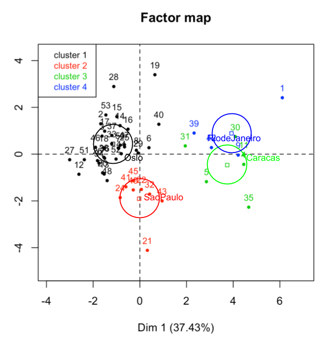
Figure 3.7: Representants of each cluster

On the first factorial plane, we observe the effect of how distances are distorted due to the shrinking of the cloud of city-points in this plane.

In certain applications, it is interesting to identify the representans of a certain category, in order to explore its attributes (for example, which are the attributes of the category men, according to the active variables of a survey).