2.5 Simultaneous Representations
2.5.1 Old Unit Axes
In a Principal Component Analysis the cloud of individuals as well as the cloud of variables are defined in different spaces, with distinct origins and distinct vector basis.
For the cloud of row-points, the origin corresponds to the center of gravity of the individuals. This space is of \(p\) dimensions and we denote \(\mathbf{u}_{\alpha}\) the corresponding base.
In turn, for the cloud of column-points the origin is the point zero. This space is of \(n\) dimensions (although the active variables define a subspace of \(p\) dimensions) and denote the factorial axes as \(\mathbf{v}_{\alpha}\).
Because the row-points and the column-points are therefore in different spaces it is impossible to simultaneously visualize them in the same space, in such a way that the inner proximities are respected (without deformations).
However, it is possible to represent the directions defined by each active variable over the base of factorial axes \(\mathbf{u}_{\alpha}\).
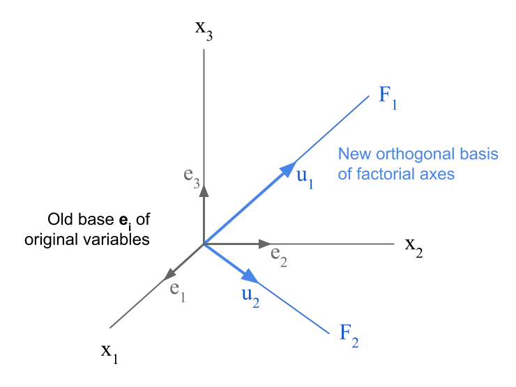
Figure 2.20: Old base in original p-dimensional space, and the new based formed by the factorial axes.
The vectors that define the directions of the original variables are the vectors \((1,0,0, \dots)\), \((0,1,0,\dots)\), \((0,0,1,0,\dots)\), etc.
Let \(\mathbf{e_j}\) be the \(j\)-th vector of this basis. Its projection on the basis determined by the vector \(\mathbf{u}_{\alpha}\) is defined by the scalar product of the vectors:
\[ \mathbf{e_j}^\mathsf{T} \mathbf{u}_{\alpha} = u_{j\alpha} \tag{2.19} \]
The element \(u_{j\alpha}\) is the \(j\)-th component of the vector \(\mathbf{u}_{\alpha}\).
The projection of the old axes, defining the directions of the active variables, over a new factorial basis, is given by the components of the eigenvectors \(\mathbf{u}_{\alpha}\) from the analysis of row-points.
We can considered an old axis \(j\)—direction of the \(j\)-th variable—as an artificial “individual” in the space of the individuals. This “individual” has a coordinate 1 in the \(j\)-th axis and 0 in the rest of the axes. In this way, the variable-point \(j\) can be located in the core of the cloud of row-points of the factorial plane. Its interpretation in straightforward: this point \(j\) is the extreme of the unit vector that defines the direction of growth of variable \(j\) in the cloud of individuals.
Interestingly, the \(p\) variables can be regarded as \(p\) unit vectors located in the core of the cloud of row-points. This involves a translation of the original basis to the average point of individuals. Obviously, these \(p\) points are on a hypersphere of unit radius.
In the first factorial plane of the cloud of individuals, these \(p\) unit vectors will be located inside a circle of unit radius as projected on the orthonormal basis of the active variables.
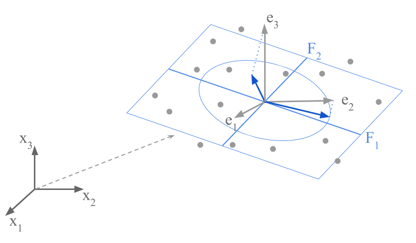
Figure 2.21: Projection of the original axes on the factorial plane with the cloud of row-points.
Notice that there is no common unit between the length 1 of the unit vector defined by the \(j\)-th variable and the values of the coordinates of the individuals over an axis. Because only the direction is what matters, we can strettch these unit vectors in such a way that the directions defined by them are clearly “readable” in the cloud of row-points.
In our working example, figure 2.22 shows the simultaneous representation of the cities and the active variables.
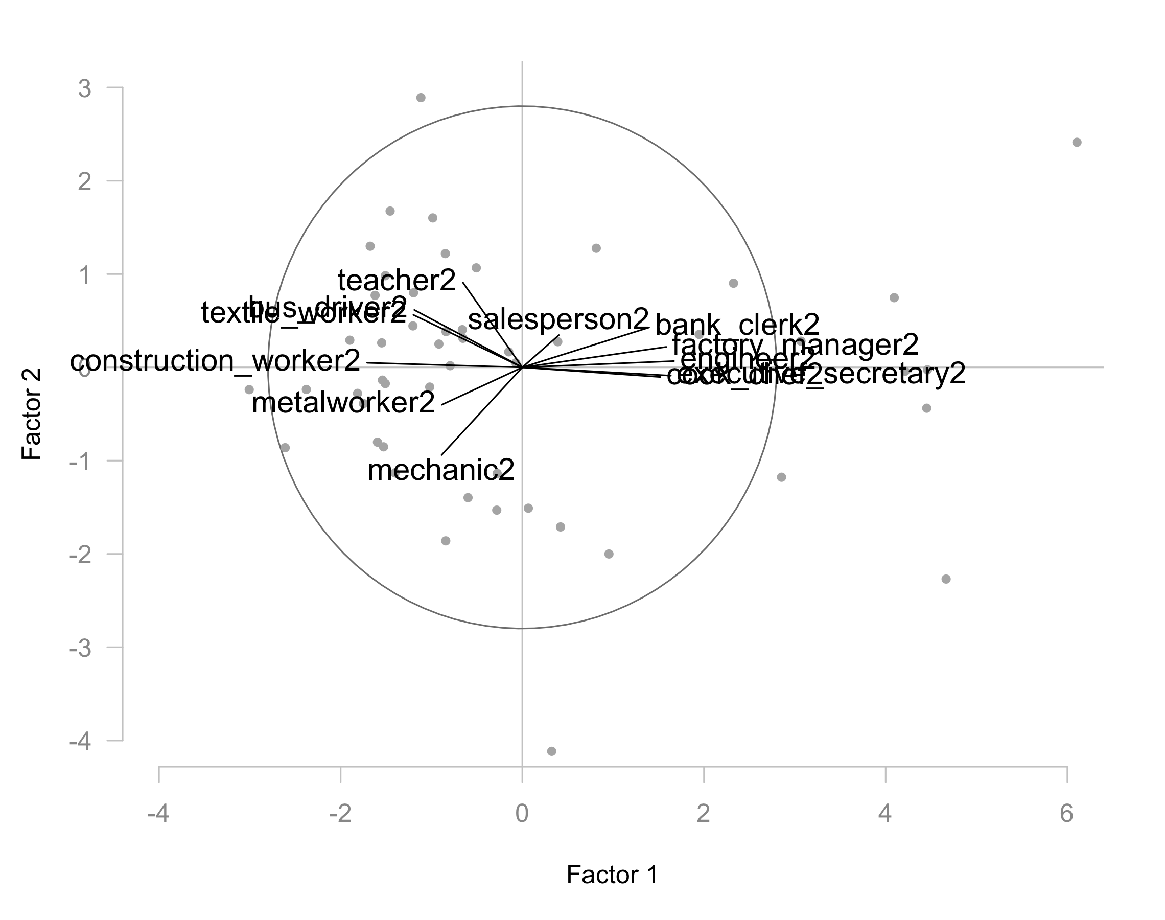
Figure 2.22: Row-points with directions of growth of the variables (old unit-vector axes).
This configuration of variable-points differs from the configuration obtained in section 2.2. Before, the angle between two variables \(j\) and \(j'\) was a measure of correlation between them. Now, all the angles are square angles; we only observe the projection of these square angles on the factorial plane.
If the arrowhead of the vector representing a variable-point is close to the circumference of radius 1, this means that the direction of growth of this variable is well defined in the factorial plane. Likewise, the individuals that are near the center take values that are close to the average of the variable. In contrast, the individuals that are further from the center, following the direction of growth of a variable, have large values for such variable.
Notice that, if in this simultaneous representation, all the unit vectors form an narrow array around the first factorial axis. This inidicates a size factor. All the variales increase—and decrease—simultaneously in the direction of the first axis.
About the representation of variable-points
The coordinate of the variable \(j\) on the axis \(\alpha\) is (see formula (2.10)):
\[ \sqrt{\lambda_{\alpha}} \hspace{1mm} u_{j \alpha} \]
The coordinate of the unit vector representing the direction of growth of variable \(j\) on the axis \(\alpha\)—in the simultaneous representation graph—is:
\[ u_{j \alpha} \]
The similarity between these two formulas implies that their respective graphic displays are also similar. The only difference is a scaling factor of \(\sqrt{\lambda_{\alpha}}\), which is visually reflected as a stretching effect.
For example, the comparison of both clouds of old and new unitary axes is shown in figure 2.23.
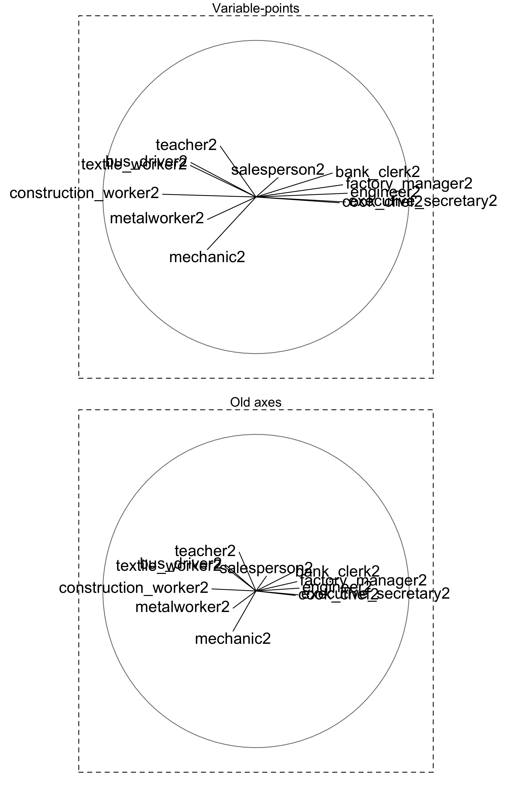
Figure 2.23: Representation of the variable-points (top) and the old axes (bottom).
This graphical similarity leads to abuse of language in interpretating simultaneous representation (mixing analysis of angles and analysis of growth directions).
Notice that it is not possible to directly display at the same time the supplementary variables in a simultaneous PCA plot of variables-individuals. The supplementary variables do not participate in the definition of the original basis for the cloud of row-points.
In Summary …
In every PCA we have two available representations of the variables:
The representation of the cloud of variable-points: each variable is a vector (unit vector if we perform a normalized PCA), and we study the angles between these vectors.
The simultaneous representation of individuals and active variables: the variable-points are the ends of the orthogonal unit vectors indicating the directions of growth of the variables.
We should say that these two representations of the variables can be regarded as two extreme situations of a more general representation system introduced by Gabriel (1971). Under this system, commonly known as biplot, the data table is decomposed as the product of two matrices: one matrix represents the rows, and the other matrix represents the columns. The biplot involves the joint representation of both elements (rows and columns) in one graphic.