4.1 Lascaux Cave Temperatures
Our first example has to do with temperatures in the famous Lascaux Cave. This grotto is a complex of caves located in the department of Dordogne in southwestern France. The cave contains over 600 parietal wall paintings, depicting large animals (e.g. bulls, bisons, ibexes, rhinoceros) from the Upper Paleolithic time period.
The control of environmental variables (e.g. temperatures measured in distinct places, hydrometry measurements, etc.) in Lascaux cave was done in a manual fashion decades ago. The measurements involved daily readings of 77 different locations in the cave. From these readings, a technical operator in charge of the machines installed in the cave, controled the settings in order to guarantee adequate environmental conditions for the conservation of the paintings.
In the late 1970s, it was acknowledged that a less manual and time consuming work for controling the environment conditions in the cave had to be implemented. The institution responsible to develop an automatic temperature controling system was the Laboratoire de Recherche des Monuments Historiques LRMH (research laboratory of historical momuments). One of the stages in this research project involved deciding whether to locate the sensors for reading temperatures along the cave.
We use a temperature data set that was part of this reserach project. The purpose is to see in what way PCA can be applied in order to describe the evolution of the cave temperatures, in terms of the reading positions, and the date of such readings. We seek to obtain a description that allows us to better understand the environment conditions of the cave. As part of this analysis, we’ll see how looking for optimal regressions enable us to select a minimum number of temperature points that capture as much of the information as possible needed to control the temperature conditions of the cave.
4.1.1 Temperature Data
The data of this section have to do with temperatures collected in 30 different locations along the cave, observed over 482 days, between February 1981 and December 1982. The following diagram shows the location of the measurements inside the cave. Each label involves a thermometer, installed either on the rock, or outside.
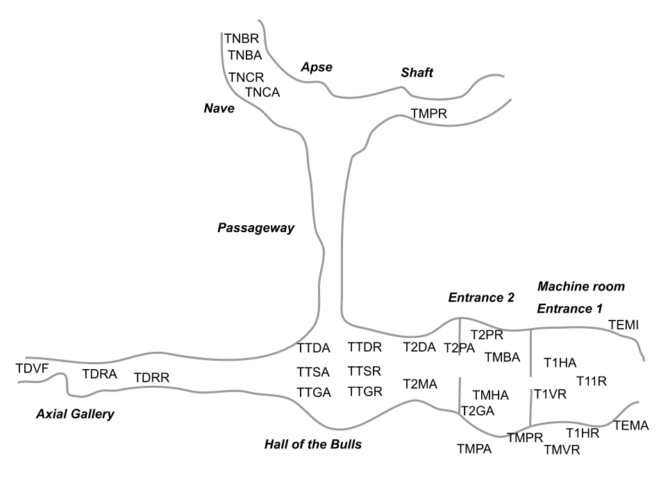
Figure 4.1: Location of reading temperature sensors
The following table lists the 30 active variables used in the analysis (continuous variables, representing temperature measurements in Celsius degrees).
| Num | Variable | Description |
|---|---|---|
| 7 | temi | Minimum outside temperature |
| 8 | tema | Maximum outside temperature |
| 9 | t11r | SAS1 left 1 - rock |
| 12 | t1ha | SAS1 left 3 up - air |
| 13 | t1hr | SAS1 left 3 up - rock |
| 14 | t1vr | SAS1 under dome 3 - rock |
| 15 | tmpa | Machine room left wall - air |
| 16 | tmpt | Machine room left wall - rock |
| 17 | tmvr | Machine room, left dome - rock |
| 18 | tmha | Machine room top wall left - air |
| 19 | tmba | Machine room bottom wall left - air |
| 20 | t2pa | SAS2 right wall - air |
| 21 | t2pr | SAS2 right wall - rock |
| 22 | t2ma | SAS2 dome - air |
| 23 | t2da | SAS2 ground right - air |
| 24 | t2ga | SAS2 ground left - air |
| 28 | ttda | Hall of the Bulls right wall - air |
| 29 | ttdr | Hall of the Bulls right wall - rock |
| 30 | ttsa | Hall of the Bulls ground - air |
| 31 | ttsr | Hall of the Bulls ground - rock |
| 32 | ttga | Hall of the Bulls left wall - air |
| 33 | ttsr | Hall of the Bulls left wall - rock |
| 34 | tdra | Axial Gallery narrow dome - air |
| 35 | tdrr | Axial Gallery narrow dome - rock |
| 36 | tdvf | Axial Gallery end dome - air |
| 37 | tnca | Nave of Deer - air |
| 38 | tncr | Nave of Deer - rock |
| 39 | tnba | Nave of Bisons - air |
| 40 | tnbr | Nave of Bisons - rock |
| 41 | tpmr | Shaft edge - rock |
Looking at the diagram of the cave in figure 4.1, the entrance is on the right side of the figure. The machine room is located below the first entrance. Then comes the Hall of the Bulls. Ahead this hall, there is the Axial Gallery. To the right of the hall, there is the passageway. As you can tell from the table of variables, all temperature readings are recorded “in the air” as well as “on the rock”.
4.1.2 PCA
We perform a first normalized Principal Component Analysis on the table of temperatures. In this analysis, we don’t take into account the time component of the measurements. In other words, we don’t take into account the date in which the readings were made. However, we do consider the time related variables (month, and year) as supplementary variables.
Looking at the table of eigenvalues in 4.2, we clearly detect two dominant axes (see table 4.2). About 50% of the variability in the first axis, and 30% of the variability in the second one. The remaining 28 axes account for the less than 20% of the total inertia. Therefore, we are confident that the first factorial plane depicts a stable configuration of associations.
| num | eigenvalue | percentage | cumulative |
|---|---|---|---|
| 1 | 14.8677 | 49.57 | 49.57 |
| 2 | 9.0366 | 30.13 | 79.69 |
| 3 | 1.8428 | 6.14 | 85.84 |
| 4 | 1.3074 | 4.36 | 90.20 |
| 5 | 0.9548 | 3.18 | 93.38 |
| 6 | 0.4578 | 1.53 | 94.91 |
| 7 | 0.3835 | 1.28 | 96.19 |
| 8 | 0.2860 | 0.95 | 97.14 |
| 9 | 0.1900 | 0.63 | 97.77 |
| 10 | 0.1010 | 0.34 | 98.11 |
| 11 | 0.0855 | 0.29 | 98.39 |
| 12 | 0.0706 | 0.24 | 98.63 |
| 13 | 0.0656 | 0.22 | 98.85 |
| 14 | 0.0564 | 0.19 | 99.04 |
| 15 | 0.0468 | 0.16 | 99.19 |
| 16 | 0.0397 | 0.13 | 99.32 |
| 17 | 0.0353 | 0.12 | 99.44 |
| 18 | 0.0314 | 0.10 | 99.55 |
| 19 | 0.0269 | 0.09 | 99.64 |
| 20 | 0.0215 | 0.07 | 99.71 |
| 21 | 0.0143 | 0.05 | 99.76 |
| 22 | 0.0140 | 0.05 | 99.80 |
| 23 | 0.0121 | 0.04 | 99.84 |
| 24 | 0.0110 | 0.04 | 99.88 |
| 25 | 0.0097 | 0.03 | 99.91 |
| 26 | 0.0070 | 0.02 | 99.94 |
| 27 | 0.0063 | 0.02 | 99.96 |
| 28 | 0.0053 | 0.02 | 99.97 |
| 29 | 0.0045 | 0.02 | 99.99 |
| 30 | 0.0033 | 0.01 | 100.00 |
Configuration of Temperature-Points
The configuration of the temperatures (active variables) in the first factorial
plane, see figure 4.2, shows a regular pattern, with arrows
close to the circumference of radius one. This means that the position of the
variables on the first plane provides a good approximation of the correlations
between the measurement points. This is less true for the exterior temperatures
(temi and tema) and for those observed in the machine room, which show a
less regular evolution, as well as a less direct association with the internal
temperatures of the cave. Notice the central position of the arrow corresponding
to the temperature near the shaft (tpmr).
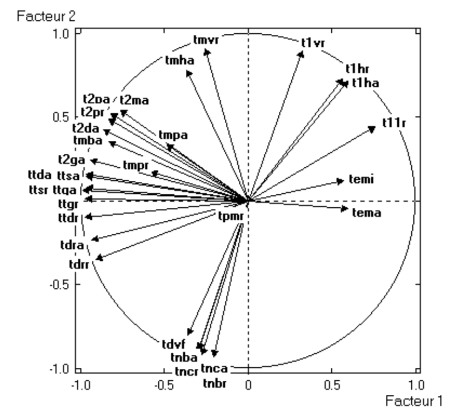
Figure 4.2: Circle of correlations.
We also see that those observation points that are physically close to each other inside the cave, are also close on the factorial plane. Which is a translation of the fact that closer readings, measure similar things (this is particularly seen among the temperatures “in the air” that always appear next to the temperatures “on the rock”).
Likewise, we observe that temperatures are scattered all around the
circumference in a counterclockwise direction: starting from the variables
that have to do with the external temperature (temi and tema), and then
moving “upward” with the variables corresponding to the readings of the
entrance in the cave, followed by the readings from the Hall of the Bulls
which are in an opposite direction to the external temperatures. Finally, we
observe the readings from the axial gallery, and then the readings from the
nave and the shaft.
This configuration reflects the effect of “distance from the cave’s entrance”. The farther from the entrance, the less the correlation of a given reading and the reading from the external temperature, except with the readings in the Hall of the Bulls that are negatively correlated with the external temperature.
Those readings from locations near the entrance are the ones that have the most
variability. This is due to the fact that they are more influenced by the
external temperature, but also because their proximity to the machine room.
Beyond the second entrance, the associations between the temperatures become
more stable and clearly reflect the geographic proximity and distance to the
entrance. Notice that the reading of point tdvf, located at the end of the
axial gallery, behaves in a similar fashion as those readings located in the
nave.
The only exception to the previous pattern is the temperature of the shaft. According to the experts, the system of temperatures in this location is independent from what happens in the rest of the cave, because of the presence of carbonic gas under the surface. The temperatures of the machine room seem to be relatively far from the circumference, which is explained by the closeness of the sensors to the machines.
4.1.3 Seasonal Phenomenon
As we previously mentioned, the data collected in the Lascaux Cave involves temperatures measured in 30 different locations along the cave, observed over 482 days, between February 1981 and December 1982.
So far, we have presented the results of the variables, that is, the results from analyzing the 30 temperature readings. However, we also have the 482 days that correspond to the rows of the data table (i.e. the individuals). In other words, we also have the 482 points that correspond to the cloud of row-points.
As we know, two days will appear close to each other if their 30 temperatures are similar. Conversely, if two days have very different temperatures, they will appear far from each other (the more different their profiles, the farther they will be). In order to better visualize the scatterplot of the cloud of points, we calculate the monthly averages, obtaining 23 points, from February 1981 to December 1982 (see figure 4.3).
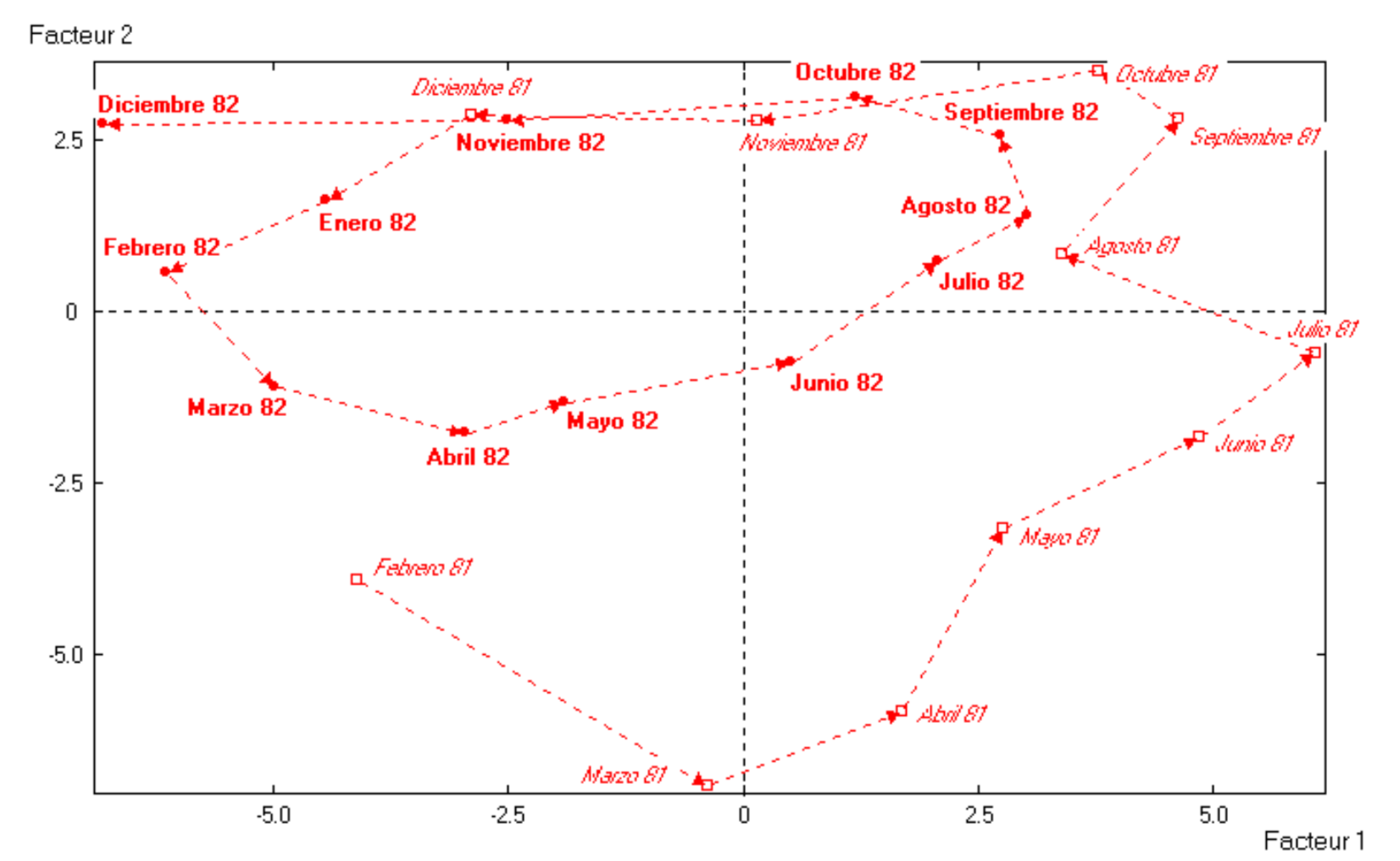
Figure 4.3: Average monthly temperature values in Lascaux Cave
As you can tell from this scatterplot, we have connected all consecutive months with a dotted line, starting in Feb-1981, and following the direction of the arrows till the last point in Dec-1982. It is interesting to see that the connected points form two loops. One loop for points of 1981, which is the outer loop; and another loop for points of 1982, which is narrower and offset to the left from the center of the plane.
It seems that the factorial plane describe the transition of the year seasons, in a counterclockwise manner. The first axis opposes Summer months to Winter months. In turn, the second axis opposes Spring months to Fall months.
In addition, we observe that, from the interior of the cave, the years 1981 and 1982 are not that similar with respect to the monthly temperatures. 1981 seems to have a hotter Summer and colder Winter, whereas in 1982 the seasons are less different, and overall, less cold. This has been confirmed by checking the records from local weather stations.
Thermal Wave Penetration
We can now take a look at both graphs (4.2 and 4.3) and enrich the interpretation of results. The configuration of the temperatures in the circle of correlations, and the pattern of the monthly temperatures, reveal the penetration of the thermal wave inside the cave.
We are able to observe how temperature changes and moves inside the cave. The high temperatures of July and August, move from the exterior towards the first entrance during the months of September and October. By Fall, the maximum recorded temperatures occur in the second entrance (October and December). Then, in Winter (January, February, and March) the maximum temperatures are recorded in the Hall of the Bulls. The further we go into the cave, the more we advance in time (from the thermal point of view). The factorial plane allows us to visualize the average time that the thermal wave takes to reach every recording location in the cave.
4.1.4 Modeling Propagation of Thermal Wave
The discovered patterns of variability in the cave’s temperature and the thermal wave, suggests us a modeling approach based on two aspects: 1) the factorial plane shows that each month corresponds to an almost constant rotation; 2) on the circle of correlations, the variables are positioned in terms of their distance from the entrance to the cave.
Let’s consider the variation of the temperature to be modeled with a sine curve. The penetration of the thermal wave in the cave is a function of the distance between two reading-temperature locations. Let \(i\) be the day, and let \(j\) be the distance to the entrance. Also, the amplitude of variation varies according to the year (coefficients \(\alpha_1\) and \(\alpha_2\)), as well as the average annual temperature (\(\mu_1\) and \(\mu_2\)).
We model the temperature of the first year, in day \(i\), and with a distance \(j\) to the entrance, with the following equation:
\[ T_1(i,j) = \alpha_1 \sin \big( 2\pi (i+j) \big) + \mu_1 \]
Analogously, the equation for the second year is:
\[ T_2(i,j) = \alpha_2 \sin \big( 2\pi (i+j) \big) + \mu_2 \]
It can be shown that, in a data table that has these relationships, the following properties are verified:
If the amplitudes and the annual means are equal, we obtain two non-null identical eigenvalues. The temperatures are ordered by a subindex on the circle of correlations, and the months progress in chronological order, confounded for both years on the same circumference (see diagram A in figure 4.4).
If there is a difference between the annual temperature means (\(\mu_1\) and \(\mu_2\)), the clouds of 1981 and 1982 become separated. If the difference is not too large, then the two first eigenvalues are similar, whereas the third eigenvalue is much more small. In turn, the months will be arranged in an elliptical way, with two off-centered ellipses (see diagram B in figure 4.4). If the difference between the annual means is more substantial, the first axis will be a function of this difference (see diagram C in figure 4.4), while in the second and third axes, the annual circumferences that are identical will be displayed.
If additionally, there is a difference of annual amplitude (\(\alpha_1\) and \(\alpha_2\)), then the size of the ellipses is modified.
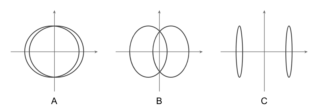
Figure 4.4: Three shape patterns of month-points
Reconstitution of the Data
Without loss of generality, let us simplify things a bit by assuming that the data table has weekly observations, instead of daily observations. The year 1981 involves weeks \(i = 1, 2, \dots, 52\), and year 1982 involves weeks \(i = 53, 54, \dots, 104\). Based on the original data, we take \(\mu_1 - \mu_2 = 0.7\), and set amplitudes to \(\alpha_1 = 1\) and \(\alpha_2 = 1.5\). For the \(j\)-th variable, we define the distance between reading points according to their groupings in the cave, except for the first 8 reading locations for which we introduce a variable distance (see table below) that corresponds to the sepration of the reading points in the entrances and the machine room.
| j | d |
|---|---|
| week | distance |
\[ \begin{array}{c|c} j & \text{distance} \\ \hline \text{1 to 8} & 2\pi (j - 8) / 21 \\ \text{9 to 15} & \pi / 3 \\ \text{16 to 25} & \pi / 2 \\ \text{26 to 30} & \pi \end{array} \]
Analyzing the weekly data table previously described, we obtain a configuration of points very similar to the one obtained with the original data. There is a big loop for 1981, and a smaller loop for 1982, off-centered and overlaping with the big loop in the winter zone. The inertia percentages of the first three axes are: 59%, 31%, and 14%, very similar to the original inertias. This indicates that the chosen model is acceptable.
4.1.5 Stability of the Axes
The histogram of eigenvalues suggests a good stability of the first two axes. This is due to the existance of the seasonal phenomenon.
To determine the number of stable axes, we add random noise to the data. The “important” axes must remain (for the most part) unchanged by the added noise, as long as they convey the structural relationships between data points.
As an illustration, let’s review how a large random noise (of up to 50% of the variability in the series) is not enough to destroy the seasonal structure in data, while remaining stable in the first two axes.
The way we add random noise to data is by adding a random amount generated from a Normal distribution, using mean zero, and standard deviation of 1/4 the standard deviation of the annual temperatures in a given reading location. We perform PCA on this modified data set, examining the obtained principal components, as well as the circle of correlations between the original components and the ones obtained from the data with random noise (see table below).
| random1 | random2 | random3 | random4 | random5 | |
|---|---|---|---|---|---|
| original1 | 0.996 | ||||
| original2 | 0.019 | 0.994 | |||
| original3 | 0.000 | 0.013 | 0.974 | ||
| original4 | 0.002 | 0.000 | 0.027 | 0.921 | |
| original5 | 0.003 | 0.006 | 0.006 | 0.043 | 0.92 |
It turns out that with this added random noise, the first five axes remain stable.
Next, we repeat the same procedure, but this time adding a larger amount of random noise: half of the standard deviation of each variable (see results in table below).
| random1 | random2 | random3 | random4 | random5 | |
|---|---|---|---|---|---|
| original1 | 0.986 | ||||
| original2 | 0.039 | 0.975 | |||
| original3 | 0.000 | 0.025 | 0.908 | ||
| original4 | 0.003 | 0.000 | 0.057 | 0.761 | |
| original5 | 0.005 | 0.011 | 0.016 | 0.064 | 0.751 |
Despite the larger amount of introduced random noise, the first three axes still remain mostly unchanged, whereas the fourth and the fifth axes have been slightly modified.
4.1.6 Selecting Best Temperature Reading Locations
As we mentioned in the introduction of this chapter, one of the stages of the Lascaux Cave research project involved deciding whether to locate the sensors for reading temperatures along the cave.
We seek to obtain a small subset of reading locations, such that they provide essential information for the totality of the observations. Simply put, we seek to conserve the stable factorial directions.
The first decision that we made was to retain just one of the measurements for every pair of temperature “rock/air”; this reduced the number of readings from 30 to 15 temperature variables.
We provide only the sketch idea used to find the solution. The methodology consists of eliminating, step by step, the more redundant variables. We use the correlation between the new computed factorial axes (PCA on retained temperature reading locations) and the original factorial axes (PCA on all variables). To be more precise, we calculate the sum of squared correlations between homologous axes (diagonal of the correlation matrix). Finally, we obtain a subset of 8 variables that adequately reconstitute the subspace of the first three initial factorial axes (with correlations of 0.986, 0.980, and 0.865, like in the table 4.6 below).
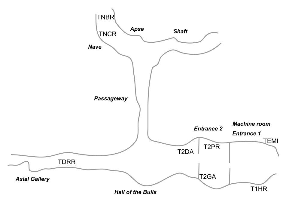
Figure 4.5: Location of best 8 reading temperature sensors
| random1 | random2 | random3 | |
|---|---|---|---|
| original1 | 0.986 | ||
| original2 | 0.162 | 0.980 | |
| original3 | 0.046 | 0.008 | 0.865 |