2.1 Principal Components
Let’s consider the cloud of row-points, also known as the cloud of individuals. As we’ve mentioned, we are interested in decomposing the inertia (i.e. the spread) of this cloud in terms of a series of orthogonal directions.
The first step consists of looking for the most basic type of subspace, namely, a line. Geometrically, a line can be defined by a vector \(\mathbf{u}\) of unit norm. Based on the discusion from the previous chapter, we will attempt to define \(\mathbf{u}\) in such a way that the projected points on this direction have maximum inertia (see figure 2.1). In other words, \(\mathbf{u}\) will be defined such that the distances between pairs of projected points are as close as possible to the original distances.
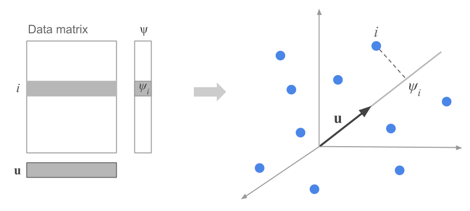
Figure 2.1: Projection of a row-point on the direction defined by a unit vector
The projection (or coordinate) of a row-point on the direction defined by \(\mathbf{u}\) is given by:
\[ \psi_i = \sum_{j=1}^{p} (x_{ij} - \bar{x}_j) u_j \tag{2.1} \]
The inertia (or variance) of all the projected points on \(\mathbf{u}\) is then:
\[ \sum_{i=1}^{n} = p_i \hspace{1mm} \psi_{i}^{2} = \lambda \tag{2.2} \]
The goal is to look for a line \(\mathbf{u}\) that maximizes the value \(\lambda\).
Let \(\mathbf{X}\) be the mean-centered data matrix. Obtaining \(\mathbf{u}\) implies diagonalizing the cross-product matrix \(\mathbf{X^\mathsf{T} X}\). This matrix is the correlation matrix in a normalized PCA, whereas in a non-normalized PCA this matrix becomes the covariance matrix.
It turns out that the unit vector \(\mathbf{u}\) is the eigenvector associated to the largest eigenvalue from diagonalizing \(\mathbf{X^\mathsf{T} X}\).
Analogously, the orthogonal direction to \(\mathbf{u}\) that maximizes the projected inertia in this new direction corresponds to the eigenvector associated to the second largest eigenvalue from diagonalizing \(\mathbf{X^\mathsf{T} X}\). This maximized inertia is equal to the second eigenvalue, so on and so forth.
The eigenvalues provide the projected inertias on each of the desired directions. Moreover, the sum of the eigenvalues is the sum of the inertias on the orthogonal directions, and this sum is equal to the global inertia of the cloud of points.
| Eigenvalues | Eigenvectors |
|---|---|
| \(\lambda_1\) | \(\mathbf{u_1}\) |
| \(\lambda_2\) | \(\mathbf{u_2}\) |
| \(\dots\) | \(\dots\) |
| \(\lambda_p\) | \(\mathbf{u_p}\) |
\[ I_T = \lambda_1 + \lambda_2 + \dots + \lambda_p = \begin{cases} p & \text{in normalized PCA} \\ & \\ \sum_{j=1}^{p} var(j) & \text{in non-normalized PCA} \end{cases} \tag{2.3} \]
The eigenvectors give the directions of maximum inertia and we call them factorial axes.
On these directions we project the individuals, obtaining what is called the principal components (see formula (2.1)). As we can tell, each component is obtained as a linear combination of the original variables:
\[ \boldsymbol{\psi}_{\alpha} = u_1 \mathbf{x_1} + \dots + u_p \mathbf{x_p} \]
Likewise, each component has a variance equal to its associated eigenvalue:
\[ var(\boldsymbol{\psi}_{\alpha}) = \lambda_\alpha \]
In summary, a Principal Component Analysis can be seen as a technique in which we go from \(p\) original variables \(\mathbf{x_j}\), each having an importance given by its variance, into \(p\) new variables \(\boldsymbol{\psi}_{\alpha}\). These new variables are linear combination of the original variables, and have an importance given by their variance which turns out to be their eigenvalues (see figure 2.2).
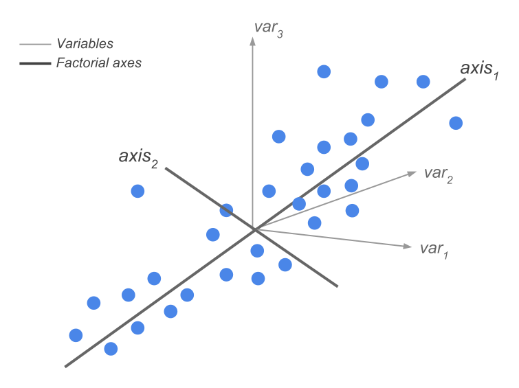
Figure 2.2: Change of basis and dimension reduction
2.1.1 Interpreting the Inertia Proportions
In our working example with the data about the cities, we obtain the following 12 eigenvalues:
| num | eigenvalues | percentage | cumulative |
|---|---|---|---|
| 1 | 10.1390 | 84.49 | 84.49 |
| 2 | 0.8612 | 7.18 | 91.67 |
| 3 | 0.3248 | 2.71 | 94.37 |
| 4 | 0.1715 | 1.43 | 95.80 |
| 5 | 0.1484 | 1.24 | 97.04 |
| 6 | 0.0973 | 0.81 | 97.85 |
| 7 | 0.0682 | 0.57 | 98.42 |
| 8 | 0.0525 | 0.44 | 98.86 |
| 9 | 0.0505 | 0.42 | 99.28 |
| 10 | 0.0332 | 0.28 | 99.55 |
| 11 | 0.0309 | 0.26 | 99.81 |
| 12 | 0.0226 | 0.19 | 100.00 |
Notice that we obtain a first principal component that stands out from the rest.
The column eigenvalue provides the explained inertia for each direction. The sum of all of the inertias corresponds to the global inertia of the cloud of cities. Observe that this global inertia is equal to 12, which is the number of variables. Recall that this is property from a normalized PCA.
The column percentage, in turn, expresses the porpotion of the explained inertia by each axis. As we can tell from the table, the first direction explains about 85% of the global inertia, which is contained in a 12-dimensional space. Because of the very large value of this principal component, one could be tempted to neglect the rest of the components. However, we’ll see that such an attitude is not excempt of risks. This does not imply that the rest of the components are useless or uninteresting. Quite the opposite, they may help reveal systematic patterns of variation in the data.
The last column of table 2.1 provides the cumulative percentage of inertia. With the first three factorial axes we summarize about 95% of the inertia (or spread) of the cloud of points.
2.1.2 How many axes to retain?
From the previous results, we’ve seen that with the first principal components, we get to recover or capture most of the spread in the cloud of points. A natural question arises: How many axes should we keep?
This is actually not an easy question, and the truth is that there is no definitive answer. In order to attempt answering this question, we have to consider another inquiry: What will the axes be used for? Let’s see some examples.
Example 1. One possibility involves using the axes to obtain a simple graphic representation of the data. In this case, the conventional number of axes to retain is 2, which are used to graph a scatter diagram: say we call these axes \(F_1\) and \(F_2\). With a third axis, we could even try to get a three-dimensional representation (\(F_1\), \(F_2\), and \(F_3\)). Beyond three dimensions, we can’t get any visual representations.
Optionally, we could try to look at partial displays of the \(p\)-dimensional space. For instance, we can get a scatterplot with \(F_2\) and \(F_3\), and then another scatterplot with \(F_1\) and \(F_4\). Keep in mind that all these partial views require a considerable “intelectual” effort. Why? Because of the fact that in any of these partial configurations, the distances between points come from compressed spaces in which some directions have dissapeared. If the goal is to simply obtain a two-dimensional visualization, it usually suffices with looking at the first factorial plane (\(F_1\) and \(F_2\)). To look “beyond” this plane, we will use outputs from clustering methods.
Example 2. If the purpose is to keep the factorial axes as an intermediate stage of a clustering procedure, then this changes things drastically. In this situation, we want to retain several axes (so that we get to keep as much of the spread of the original variables). Usually we would discard those directions associated to the smallest eigenvalues. The reason to do this is because such directions typically reflect random fluctuations—“noise”—and not really a signal in the data.
Example 3. If the goal is to use the factorial axes as explanatory variables in a regression model or in a classification model, we will try to keep a reduced number of axes, although not necessarily the first ones. It is certainly possible to find discriminant directions among axes that are not in the first positions.
As you can tell, deciding on the number of axes to retain is not that simple. This is a decision that is also linked to the stability of results.
We recommend not to blindly trust in automatic rules of thumb for deciding the number of directions to be kept. Our experience tells us that it is possible to find stable factorial axes with relatively small eigenvalue.
Note: To decrease the percentage of inertia of each axis, one can add new uncorrelated variables to the data table (i.e. white noise). Doing so should not have an effect on the first factorial axes, which should still be able to capture most of the summarized “information”.
2.1.3 Coordinates of row-points
The table below contains the results about the cities with respect to the first two factorial axes:
| city | wgt | disto | coord1 | coord2 | contr1 | contr2 | cosqr1 | cosqr2 | |
|---|---|---|---|---|---|---|---|---|---|
| 1 | AbuDhabi | 1.96 | 27.16 | 2.17 | 4.61 | 0.91 | 48.42 | 0.17 | 0.78 |
| 2 | Amsterdam | 1.96 | 3.22 | 1.58 | -0.36 | 0.48 | 0.29 | 0.77 | 0.04 |
| 3 | Athens | 1.96 | 4.24 | -1.91 | -0.51 | 0.71 | 0.58 | 0.86 | 0.06 |
| 4 | Bangkok | 1.96 | 9.87 | -2.97 | 0.82 | 1.71 | 1.53 | 0.89 | 0.07 |
| 5 | Bogota | 1.96 | 7.14 | -2.47 | 0.66 | 1.18 | 0.99 | 0.86 | 0.06 |
| 6 | Mumbai | 1.96 | 21.11 | -4.56 | -0.31 | 4.03 | 0.22 | 0.99 | 0.00 |
| 7 | Brussels | 1.96 | 0.74 | 0.61 | -0.17 | 0.07 | 0.07 | 0.50 | 0.04 |
| 8 | Budapest | 1.96 | 17.74 | -4.19 | -0.24 | 3.39 | 0.13 | 0.99 | 0.00 |
| 9 | BuenosAires | 1.96 | 5.39 | -0.89 | 1.23 | 0.15 | 3.43 | 0.15 | 0.28 |
| 11 | Caracas | 1.96 | 18.07 | -4.24 | -0.06 | 3.48 | 0.01 | 1.00 | 0.00 |
| 12 | Chicago | 1.96 | 23.64 | 4.42 | -1.25 | 3.77 | 3.55 | 0.82 | 0.07 |
| 13 | Copenhagen | 1.96 | 7.43 | 2.37 | -0.83 | 1.09 | 1.58 | 0.76 | 0.09 |
| 14 | Dublin | 1.96 | 0.79 | -0.27 | -0.19 | 0.01 | 0.08 | 0.10 | 0.05 |
| 15 | Dusseldorf | 1.96 | 8.32 | 2.72 | 0.24 | 1.43 | 0.13 | 0.89 | 0.01 |
| 16 | Frankfurt | 1.96 | 10.12 | 3.05 | 0.63 | 1.80 | 0.90 | 0.92 | 0.04 |
| 17 | Geneva | 1.96 | 42.20 | 6.36 | -0.30 | 7.82 | 0.21 | 0.96 | 0.00 |
| 18 | Helsinki | 1.96 | 0.49 | 0.03 | -0.51 | 0.00 | 0.60 | 0.00 | 0.53 |
| 19 | Hongkong | 1.96 | 3.61 | -1.03 | 0.54 | 0.21 | 0.66 | 0.30 | 0.08 |
| 20 | Houston | 1.96 | 15.21 | 3.45 | -0.78 | 2.30 | 1.37 | 0.78 | 0.04 |
| 21 | Jakarta | 1.96 | 16.92 | -4.08 | -0.20 | 3.22 | 0.09 | 0.98 | 0.00 |
| 22 | Johannesburg | 1.96 | 4.88 | -2.08 | -0.02 | 0.84 | 0.00 | 0.88 | 0.00 |
| 24 | Lagos | 1.96 | 23.54 | -4.81 | -0.43 | 4.47 | 0.42 | 0.98 | 0.01 |
| 25 | Lisbon | 1.96 | 5.00 | -2.17 | -0.28 | 0.91 | 0.18 | 0.94 | 0.02 |
| 26 | London | 1.96 | 0.76 | -0.02 | -0.63 | 0.00 | 0.91 | 0.00 | 0.52 |
| 27 | LosAngeles | 1.96 | 18.89 | 3.64 | -1.80 | 2.57 | 7.39 | 0.70 | 0.17 |
| 28 | Luxembourg | 1.96 | 32.79 | 5.24 | 0.69 | 5.30 | 1.07 | 0.84 | 0.01 |
| 29 | Madrid | 1.96 | 0.89 | -0.06 | 0.00 | 0.00 | 0.00 | 0.00 | 0.00 |
| 30 | Manama | 1.96 | 7.17 | -0.82 | 2.05 | 0.13 | 9.60 | 0.09 | 0.59 |
| 31 | Manila | 1.96 | 16.51 | -4.05 | -0.03 | 3.17 | 0.00 | 0.99 | 0.00 |
| 32 | Mexico | 1.96 | 8.63 | -2.83 | -0.07 | 1.55 | 0.01 | 0.93 | 0.00 |
| 33 | Milan | 1.96 | 0.69 | 0.02 | -0.34 | 0.00 | 0.26 | 0.00 | 0.17 |
| 34 | Montreal | 1.96 | 5.68 | 2.17 | -0.77 | 0.91 | 1.34 | 0.83 | 0.10 |
| 35 | Nairobi | 1.96 | 23.45 | -4.82 | -0.26 | 4.50 | 0.15 | 0.99 | 0.00 |
| 36 | NewYork | 1.96 | 23.01 | 4.60 | -0.30 | 4.09 | 0.20 | 0.92 | 0.00 |
| 37 | Nicosia | 1.96 | 3.56 | -1.78 | -0.27 | 0.61 | 0.16 | 0.89 | 0.02 |
| 38 | Oslo | 1.96 | 3.98 | 1.66 | -0.73 | 0.53 | 1.21 | 0.69 | 0.13 |
| 39 | Panama | 1.96 | 5.97 | -2.22 | 0.62 | 0.96 | 0.88 | 0.83 | 0.06 |
| 40 | Paris | 1.96 | 5.31 | 1.65 | 1.41 | 0.53 | 4.50 | 0.51 | 0.37 |
| 41 | Prague | 1.96 | 18.69 | -4.29 | -0.31 | 3.56 | 0.22 | 0.98 | 0.01 |
| 42 | RiodeJaneiro | 1.96 | 12.22 | -3.40 | 0.28 | 2.24 | 0.18 | 0.95 | 0.01 |
| 43 | SaoPaulo | 1.96 | 10.33 | -3.18 | -0.01 | 1.96 | 0.00 | 0.98 | 0.00 |
| 44 | Seoul | 1.96 | 0.69 | -0.61 | -0.04 | 0.07 | 0.00 | 0.54 | 0.00 |
| 45 | Singapore | 1.96 | 2.64 | -1.16 | -0.16 | 0.26 | 0.06 | 0.51 | 0.01 |
| 46 | Stockholm | 1.96 | 2.16 | 0.67 | -0.98 | 0.09 | 2.20 | 0.21 | 0.45 |
| 47 | Sidney | 1.96 | 0.62 | 0.03 | -0.21 | 0.00 | 0.10 | 0.00 | 0.07 |
| 48 | Taipei | 1.96 | 6.07 | 1.64 | -0.27 | 0.52 | 0.17 | 0.45 | 0.01 |
| 49 | Tel-Aviv | 1.96 | 3.35 | -1.41 | 0.00 | 0.38 | 0.00 | 0.59 | 0.00 |
| 50 | Tokyo | 1.96 | 46.73 | 6.72 | 0.72 | 8.72 | 1.18 | 0.97 | 0.01 |
| 51 | Toronto | 1.96 | 4.86 | 1.77 | -1.06 | 0.60 | 2.53 | 0.64 | 0.23 |
| 52 | Vienna | 1.96 | 4.07 | 1.86 | -0.11 | 0.67 | 0.03 | 0.85 | 0.00 |
| 53 | Zurich | 1.96 | 65.45 | 7.90 | 0.29 | 12.08 | 0.20 | 0.95 | 0.00 |
The column wgt indicates the weight of each city, which in this case is a
uniform weight of 100 / 51 = 1.96.
The column disto provides the squared distance of each city to the center of
gravity. This column allows us to find which cities are the typical cities
(i.e. the closest ones to the center of gravity), such as Helsinki. Likewise,
it allows us to identify the unusual or unique cities (i.e. those that have
a large distance to the center of gravity) like Zurich or Tokyo. In general,
the distance to the center of gravity is a criterion of the singularity of
each city.
The third and fourth columns correspond to the coordinates obtained from projecting the cities onto the first two factorial axes. The representation on the first factorial plane is obtained with these coordinateas (\(F_1\) and \(F_2\)), given in figure 1.9.
It is important to mention that the orientation of a factorial axis is arbitrary: the important trait is the direction. We could change the orientation of an axis by changing the sign of the coordinates on this axis. Graphically, this means that all symmetries are possible. The user has to make the decision of which orientation is the most convenient.
2.1.4 Interpretation Tools
Contributions
The next two columns, contr1 and contr2, provide the contributions (in percentages) of the cities to the explained inertia by each axis. The inertia of an axis is obtained via formula (2.2). Thus, we can measure the part of an axis’ inertia that is due to a given row-point by means of the quotient:
\[ CTR(i, \alpha) = \frac{p_i \psi^{2}_{i \alpha}}{\lambda_{\alpha}} \times 100 \tag{2.4} \]
The above quotient is the contribution of a point \(i\) to the construction of axis \(\alpha\).
We can use the contributions to identify the cities that contribute the most to the construction of the factorial axes.
If all cities had the same contribution, this would have a value of about 2% (100/51). Consequently, all those cities with contributions greater than 2% can be considered to have influence above the average.
When is a contribution considered to be “high”?
The answer to this question is not straightforward. A contribution will be considered “high” when, compared to the rest of contributions, it has an unusual large value.
For example, the city that contributes the most to the second axis is Abu Dhabi (48%). Almost half of the inertia of this axis is due to this city alone. Abu Dhabi is clearly very influent in the construction of this axis. We can actually ask about the stability of this axis, meaning, how much the result would change if Abu Dhabi were to be eliminated?
The next figure 2.3 shows the cities with a size proportional to their contributions on the first factorial plane (sum of the contributions of the first two axes).
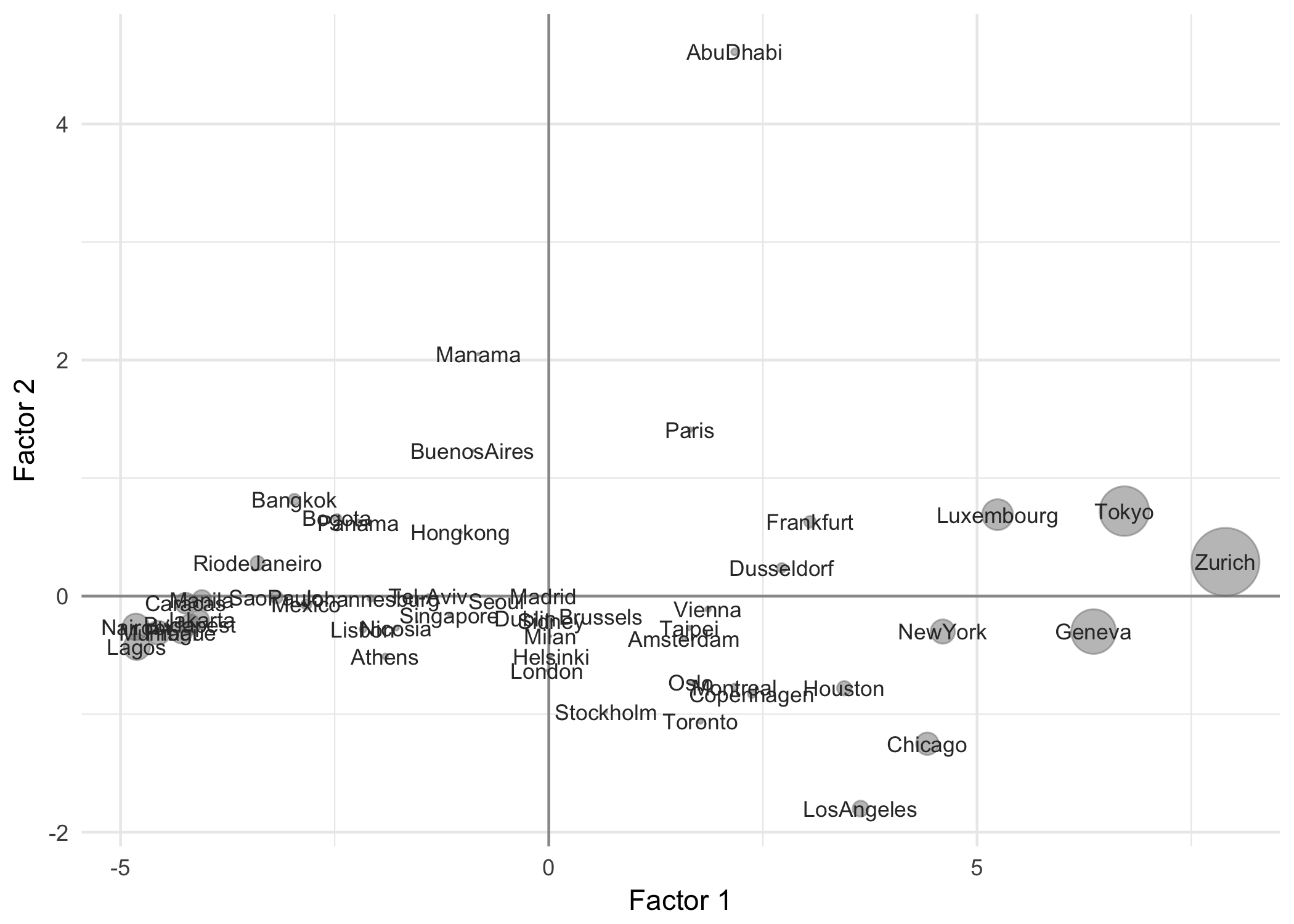
Figure 2.3: Contributions of the cities in the first factorial plane
All the active points play a role in the construction of an axis. We can check that the sum of all the contributions in an axis add up to 100.
\[ \sum_{i=1}^{n} CTR(i, \alpha) = 100 \tag{2.5} \]
Squared Cosines
The last columns of the table of results, cosqr1 and cosqr2, contain the values of the squared cosines. These are used to assess the quality of the obtained factorial configuration when compared to the original configuration of the row-points.
Because the obtained representations are an approximation of the real distances between points, it is expected that some distances between pairs of points will be better represented whereas other distances will not reliably reflect the real distance between two points.
The goal is to have a good idea of how close is a point with respect to the factorial plane. If two points are close to the factorial plane, then the projected distance will be a good approximation to the actual distance in the original space. However, if at least one point is further away from the projection plane, then the real distance can be very different from that represented in the factorial plane.
This proximity to the factorial plane is measured with the squared cosine of each point to the factorial axes.
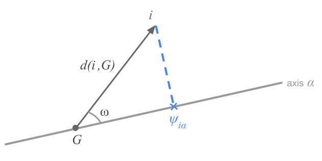
Figure 2.4: The squared cosine as a measure of proximity
The figure 2.4 illustrates the definition given in equation (2.6)
\[ COS^2(i, \alpha) = \frac{\psi^{2}_{i \alpha}}{d^2(i, G)} \tag{2.6} \]
A squared cosine of 1 means that the city is on the factorial axis (i.e. the angle \(\omega\) is zero), whereas a squared cosine of 0 indicates that the city is on an orthogonal direction to the axis.
Notice that the sum of the squared cosines over all \(p\) factorial axes is equal to 1. This has to do with fact that all axes are needed in order to have the exact position of a point in the entire space.
\[ \sum_{\alpha = 1}^{p} COS^2(i, \alpha) = 1 \tag{2.7} \]
Interestingly, the sum of the squared cosines of a given point over the first axes provides, in percentage, the “quality” of representation of the point in the subspace defined by these axes.
What value of a squared cosine indicates that a point is “well represented” on a factorial plane?
Similar to the contributions, the answer to the above question is not straightforward. A squared cosine (or the sum on the first two axes of the factorial plane) has to be compared with the rest of the squared cosines in order to determine if it is large or small.
In our working example, the cities are in general well represented on the first factorial plane. The sum of the squared cosines over the first two axes is close to 1. However, cities such as Dublin, Madrid, Sidney or Milan, which are close to the center, are not well represented. In contrast, Mumbai or Caracas are perfectly represented. Figure 2.5 shows the cities with a size proportional to their squared cosine on the first factorial plane.
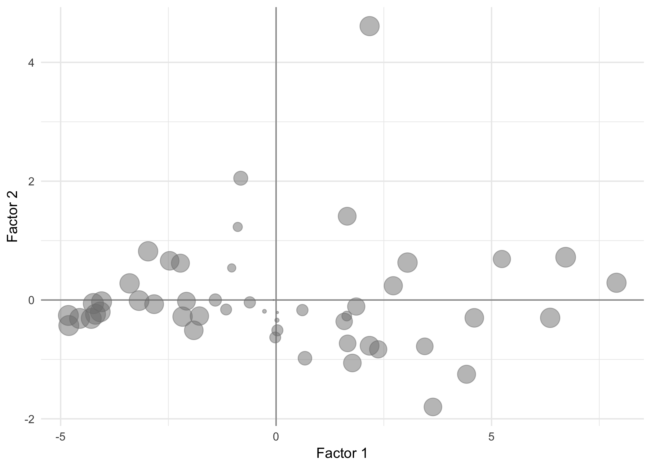
Figure 2.5: Squared cosines of the cities on the first factorial plane
The cities that are deficiently represented in this plane are the “average” cities. We can only interpret the proximity between cities if they are well represented on the factorial plane.