4.2 Design of Experiments and PCA
Our second example has to do with material coatings degrading over time that need to be replaced with protection coverings, paint, or chemical filters. We are interested in studying the effect of three factors associated with the aging of material coatings. To do this, an experimental design is carried out with the following factors:
| Factor | Levels |
|---|---|
| Radiation type | Radiation V |
| Radiation W | |
| Radiation intensity | 1/2 dose |
| 2 dose | |
| Chemical protection filter | Filter A |
| Filter B | |
| Filter C |
The material coatings go through an artifical aging process. Several parameters are measured that have to do with the apparent degradation of the surface. The experiment involves five series of measurements obtained in different times: \(\mathsf{T}_0, \mathsf{T}_1, \mathsf{T}_2, \mathsf{T}_3\) and \(\mathsf{T}_4\). The duration of the tests is of one year. In addition, we also have a series of coatings with no protection, which have been subjected to radiations in order to establish comparisons, whereas the other coatings are used as “control” units without being exposed to any radiation (only measuring their natural aging).
The observed aging parameters have been: color, thickness, lackluster, wrinkles, and cracks. We also have available an assessment of the overall aging aspect, as well as other “non controlled” variables, all of them observed as continuous variables.
4.2.1 PCA
Principal Component Analysis has been performed on a data set containing the five time periods of tests \(\mathsf{T}_0\), \(\mathsf{T}_1\), \(\mathsf{T}_2\), \(\mathsf{T}_3\), and \(\mathsf{T}_4\) (i.e. each coating is repeated 5 times). The table also contains, as nominal variables, the variable that indicates the period and the interactions with the factors of interest (radiation type, radiation dose, and type of chemical filter). The active variables are the 5 aging measurement parameters. All of the variables are listed in the following table:
| Variable | Type | Scale |
|---|---|---|
| Radiation type | supplementary nominal | 6 categories |
| Radiation dose | supplementary nominal | 4 categories |
| Protection filter | supplementary nominal | 6 categories |
| Time period | supplementary nominal | 5 categories |
| Color | active continuous | continuous |
| Lackluster | active continuous | continuous |
| Cracks | active continuous | continuous |
| Thickness | active continuous | continuous |
| Wrinkles | active continuous | continuous |
| Assessment | supplementary continuous | continuous |
Likewise, the table below shows the correlations among the active variables:
| color | lackluster | cracks | thickness | wrinkles | |
|---|---|---|---|---|---|
| color | 1.00 | ||||
| lackluster | 0.45 | 1.00 | |||
| cracks | 0.24 | 0.74 | 1.00 | ||
| thickness | 0.88 | 0.48 | 0.35 | 1.00 | |
| wrinkles | 0.60 | 0.64 | 0.57 | 0.65 | 1 |
As you can tell, all correlations are positive. This will produce a first factor with the so-called size effect, opposing the more deteriorated coatings against those that are in better shape (in the sample of size 830, we consider a non-null correlation to be 0.07, with a significance level \(\alpha = 0.05\)).
The table 4.8 shows the distribution of eigenvalues from the principal component analysis on the five aging parameters.
| num | eigenvalue | percentage | cumulative |
|---|---|---|---|
| 1 | 3.2531 | 65.06 | 65.06 |
| 2 | 1.0675 | 21.35 | 86.41 |
| 3 | 0.3284 | 6.57 | 92.98 |
| 4 | 0.2424 | 4.85 | 97.83 |
| 5 | 0.1085 | 2.17 | 100.00 |
In the figure below (circle of correlations), look at the correlation between the supplementary variable “overall assessment” and the first factor. This indicates that the first axis opposes the more degradated coatings to the less deteriorated. In turn, the second factor opposes the degradation due to lackluster and cracks, versus the degradation in color and thickness. Wrinkles are located in an intermediate position, very correlated with the overall assessment. These two factors account for 86% of the total inertia.
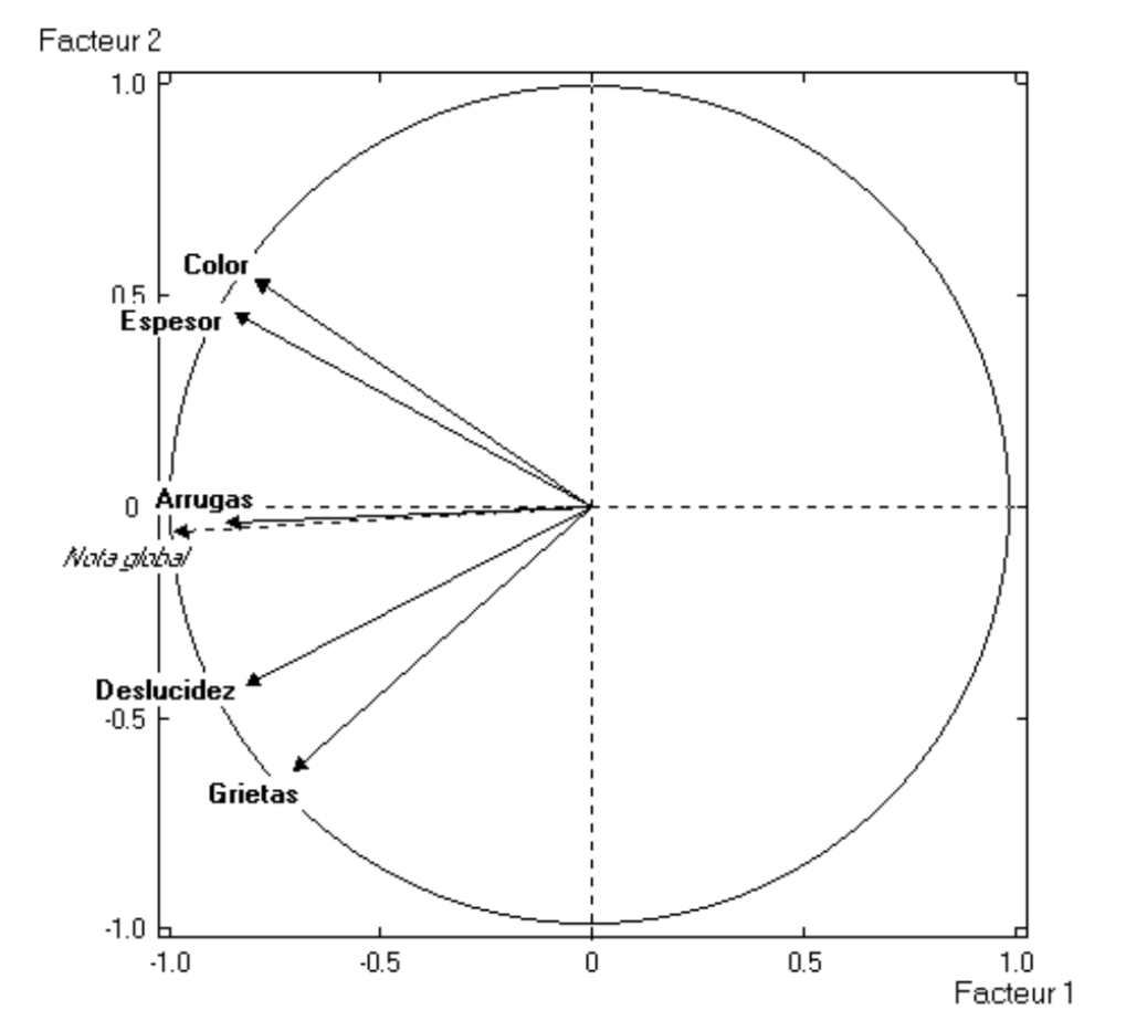
Figure 4.6: Circle of correlations for aging parameters
4.2.2 Evolution of Factor Trajectories over Time
To gain insight into the relationship between the extracted dimensions and the active variables, we project, as supplementary points, the different explanatory factors crossed with the five time periods. This operation defines trajectories in the factorial plane that help us understand the aging phenomenon under study.
We first project the different types of filters per time period, which produces trajectories fA, fB and fC in figure 4.7. We also project the non-treated coatings that have been subjected to radiation, as well as those that have not been subjected to any radiation. The latter show natural againg of the material coatings. Recall that these non-treated samples are used as control units to which we compare the different filters.
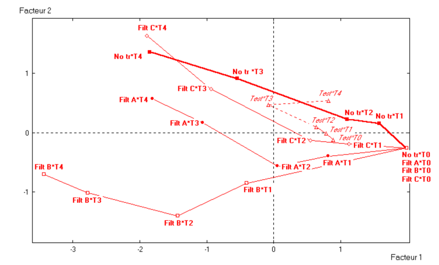
Figure 4.7: Average aging of filters per period
We observe that filter B quickly degrades coatings, especially on cracks and lackluster. In contrast, filter C has a trajectory quite close to the “non-treated” and the two time periods, close to the control samples. Then, the degradation increases, mostly in color and thickness (compare the direction of this trajectory with that of figure 4.6). With respect to filter A, this is located in an intermediate position between filters B and C.
Actually, figure 4.7 shows the average evolutions per filter, independently of the radiation type and dose.
It is interesting to project the interactions between filter type, radiation type, and radiation dose (which are the cells of the experimental design) onto the first factorial plane. Because of the large number of points to be plotted, we have divided them in two graphs. One plot contains the points for filters B and C, and the “non-treated” (figure 4.8); the other plot (see figure 4.9) contains the observations for filter A for which two types of radiation have been used: normal (1/2 dose) and high dose (2 dose).
The graph in figure 4.8 distinguishes two types of trajectories. We have a set of trajectories going from the right side of the plane to the top left corner: filter C and “non-treated”, with degradation in color and thickness. The other set of trajectories are in the left bottom part of the plane: filter B, with degradation in cracks and lackluster.
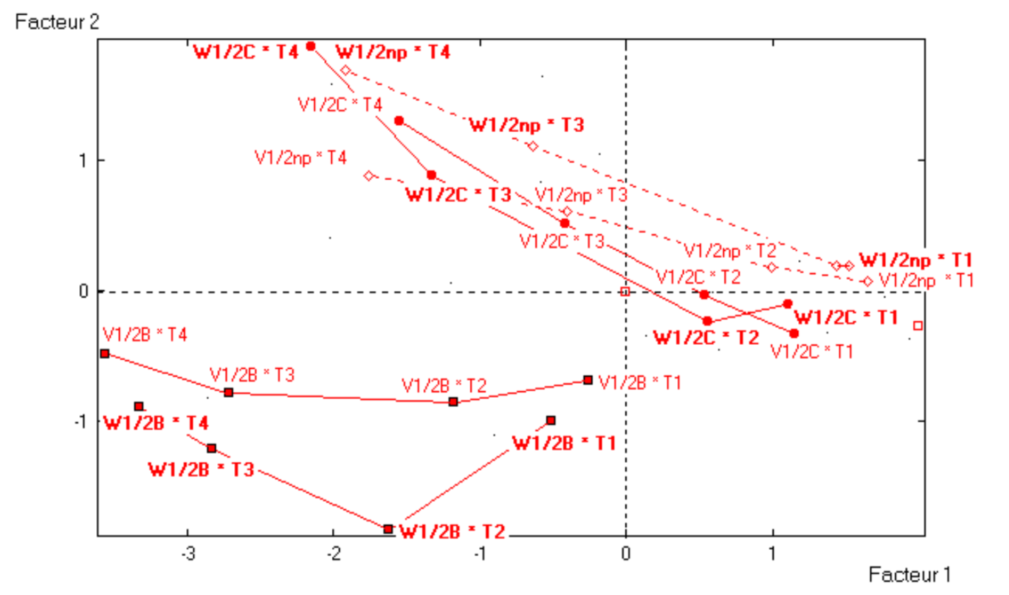
Figure 4.8: Evolution of filters B and C, according to type and dose of radiation
Note that for both, filter C and “non-treated”, there is a small divergence depending on the type of radiation, V or W. Moreover, the type of radiation W is more degradating. Likewise, filter B strongly degrades the material coating. The degradation is stronger between \(\mathsf{T}_0\) and \(\mathsf{T}_1\), and then it keeps going on but at a slower pace. Here again, the radiation W appears to be more dominant in cracks and lackluster.
With respect to filter A, we distinguish two levels of radiation intensity (dose 1/2 and 2), as well as the 2 types of radiation (V and W), shown in figure 4.9. We find that trajectory of filter A and V1/2 has a small degradation effect. In contrast, the trajectory of filter A and radiation type W behaves a lot like that of filter C and non-treated. When we move to the high dose (dose 2), the degradation of radiation V is accentuated with respect to the level that it has with lower dose (dose 1/2). However, this degradation is less than the one shown in filter B in a central position. In contrast, when we use radiation W with a dose equal to 2, then filter A behaves like filter B with the same radiation, but dose 1/2.
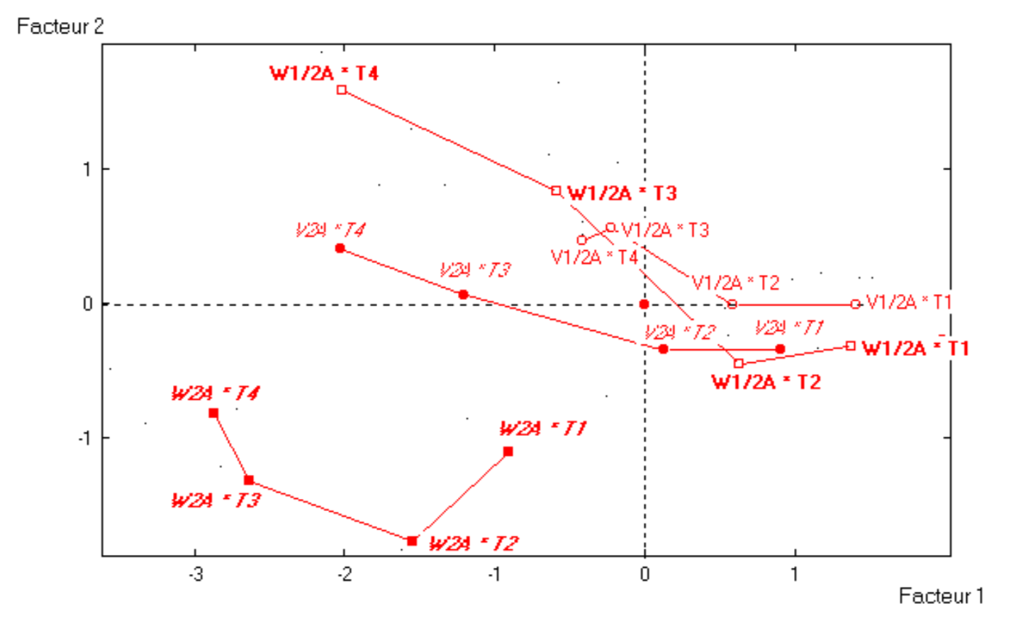
Figure 4.9: Evolution of filters A, according to type and dose of radiation
4.2.3 Analysis of Variance
We want to study how the aging of the coating surface is related with time and group. Time is expressed by the period of measurement, and the groups are defined by the combination of factors in the experimental design (interaction of filter, radiation type, and radiation dose).
We perform an analysis of variance (anova) using variable “overall assessment” as the response variable, and using period (4 dates) and group (12 combinations) as anova factors. The obtained results are displayed in table 4.9. This table contains the model’s summary statistics, and the table with the decomposition of variance.
| term | coefficient | stdev | t_stat | p_val | v_test |
|---|---|---|---|---|---|
| period T0 | -4.5940 | 0.138 | 33.262 | 0.000 | -26.42 |
| period T1 | -2.1695 | 0.138 | 15.671 | 0.000 | -14.65 |
| period T2 | -0.3717 | 0.140 | 2.665 | 0.008 | -2.66 |
| period T3 | 2.4890 | 0.142 | 17.551 | 0.000 | 16.16 |
| period T4 | 4.6463 | 0.145 | 32.000 | 0.000 | 25.74 |
| rad. V 1/2 non-treated | -0.5353 | 0.232 | 2.311 | 0.021 | -2.31 |
| rad. V 1/2 filter A | -0.7255 | 0.252 | 2.878 | 0.004 | -2.87 |
| rad. V 1/2 filter B | 3.1480 | 0.232 | 13.587 | 0.000 | 12.90 |
| rad. V 1/2 filter C | -0.2815 | 0.234 | 1.205 | 0.228 | -1.20 |
| rad. V 2 filter A | 0.8372 | 0.234 | 3.585 | 0.000 | 3.57 |
| rad. W 1/2 non-treated | -0.5601 | 0.208 | 2.696 | 0.007 | -2.69 |
| rad. W 1/2 filter A | -0.0464 | 0.207 | 0.225 | 0.822 | -0.22 |
| rad. W 1/2 filter B | 3.6387 | 0.210 | 17.299 | 0.000 | 15.96 |
| rad. W 1/2 filter C | 0.3510 | 0.207 | 1.699 | 0.090 | 1.70 |
| rad. W 2 filter A | 4.1088 | 0.270 | 15.233 | 0.000 | 14.28 |
| control | -1.5533 | 0.235 | 6.597 | 0.000 | -6.51 |
| not applicable | -8.3816 | 0.464 | 18.065 | 0.000 | -16.56 |
| constant | 8.8687 | 0.077 | 114.840 | 0.000 | 48.11 |
Residual standard error: 3260.0056 on 15 degrees of freedom
Multiple R-squared: 0.7780
F-statistic: 190.134 on 15 and 814
p-value: 0.0000
          Df    Sum Sq  F-value  Pr(>F)  v-test
Periods:   8  8574.453  535.245   0.000   32.08
Groups:   14  2886.327   88.217   0.000   42.29
We observe that both factors, time period and group, are clearly significant. The coefficients of each period are arranged in a similar fashion to the way they appear in the fatorial planes. The only positive coefficients for groups (indicating a greater degradation) are for filter B with any type of radiation, and for filter A with radiation W and dose 2.