4.3 Defining an Economic Capacity Index
Our third example has to do with assessing the mean “economic capacity” of micro metropolitan components in a given year. To be more precise, the statistical units correspond to the smallest administrative units in a big Spanish city (these units are tehnically known as “census sections”). One of the goals is to draw a map of the city showing the distribution of the economic capacity in different areas.
This type of analysis seeks to provide support in economic studies in which a geographical element is taken into account, for example, urban development projects, location of shops, services, operational branches of businesses, etc.
We will focus on the indicators about income and wealth, routinely collected by municipal data bases, and service provider companies.
Due to confidentiality issues, the treatment of the data has to be done at an aggregated level by census section. Therefore, the resulting index won’t be a family economic capacity index, but raher an estimation of the average family economic capacity by census section.
4.3.1 Analyzed Information
The analyzed information comes from four sources: municipal registry data, office of motor vehicles, municipal land registry, and telephone bills. Because the related data files contain a large number of variables, the main problem has been the selection of the variables (indicators of the economic capacity of families) to be used in the construction of the index.
The goal is to find a list of indicators in a balanced way such that all indicator subgroups have a similar importance, as well as being highly correlated.
The chosen indicators are:
First factor from a simple correspondence analysis performed on the “socioprofessional categories” of the municipal registry.
Tax potential based on car registrations.
Age of cars.
Construction value of properties (from municipal land registry)
Value of properties (from municipal land registry)
Total monthly telephone bill of all families.
These retained variables give us an idea of either the income (based on telephone bills), or the wealth (based on property values). Other variables are more complex, for instance, the tax potential of vehicles is an indicator of both income and wealth; the age of vehicles is related with renewal periods of the stock of cars; the tax value of land is associated to speculation of real estate prices, and therefore the prices of real estate in a given area. Likewise, the first factor (from a correspondence analysis of socioprofessional categories) can be interpreted as an indicator of social status in a given area.
The analyzed data are the mean values by census section. The following table shows the matrix of correlations of the described indicators.
| socioprof | cars age | land value | cars tax | dwelling value | phone bill | |
|---|---|---|---|---|---|---|
| socioprof | 1.00 | |||||
| cars age | 0.57 | 1.00 | ||||
| land value | 0.82 | 0.41 | 1.00 | |||
| cars tax | 0.67 | 0.45 | 0.71 | 1.00 | ||
| dwelling value | 0.71 | 0.65 | 0.74 | 0.71 | 1.00 | |
| phone bill | 0.74 | 0.49 | 0.75 | 0.71 | 0.76 | 1 |
4.3.2 PCA
The table 4.11, shown below, displays the distribution of eigenvalues from the principal component analysis on the six economic indicators.
| num | eigenvalue | percentage | cumulative |
|---|---|---|---|
| 1 | 4.3235 | 72.06 | 72.06 |
| 2 | 0.6800 | 11.33 | 83.39 |
| 3 | 0.3653 | 6.09 | 89.48 |
| 4 | 0.2768 | 4.61 | 94.09 |
| 5 | 0.2315 | 3.86 | 97.95 |
| 6 | 0.1230 | 2.05 | 100.00 |
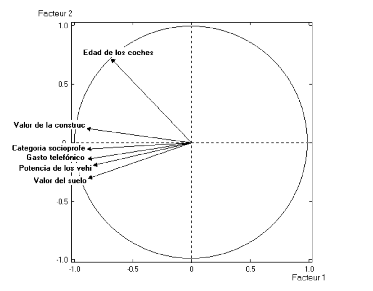
Figure 4.10 depicts the circle of correlations. Note how all variables, except “age of vehicles”, are highly correlated with the first axis. This reflects the so-called size effect. The amount of inertia captured by the first axis is 72% (of the total inertia).

Figure 4.10: Circle of correlations of economic indicators
The correlations of the original variables with the first principal component are as follows:
| Variable | Correlation |
|---|---|
| Value of properties | 0.90 |
| Socioprofessional category | 0.89 |
| Construction value | 0.88 |
| Telephone bill | 0.88 |
| Tax potential based on car | 0.84 |
| Age of vehicles | 0.68 |
As you can tell, these are high correlations, which indicates that the first factor is a good representant of all the analyzed variables. These correlations give the coefficients for the explanatory model using the first factor (assuming mean-centered and reduced variables). The fact that most of the coefficients are very similar, implies that the first factor is a good approximation to the arithmetic mean of the variables. Consequently, the first principal component allows us to order the census sections according to their level of economic capacity. The centroid of this factor corresponds to the average economic capacity of the city.
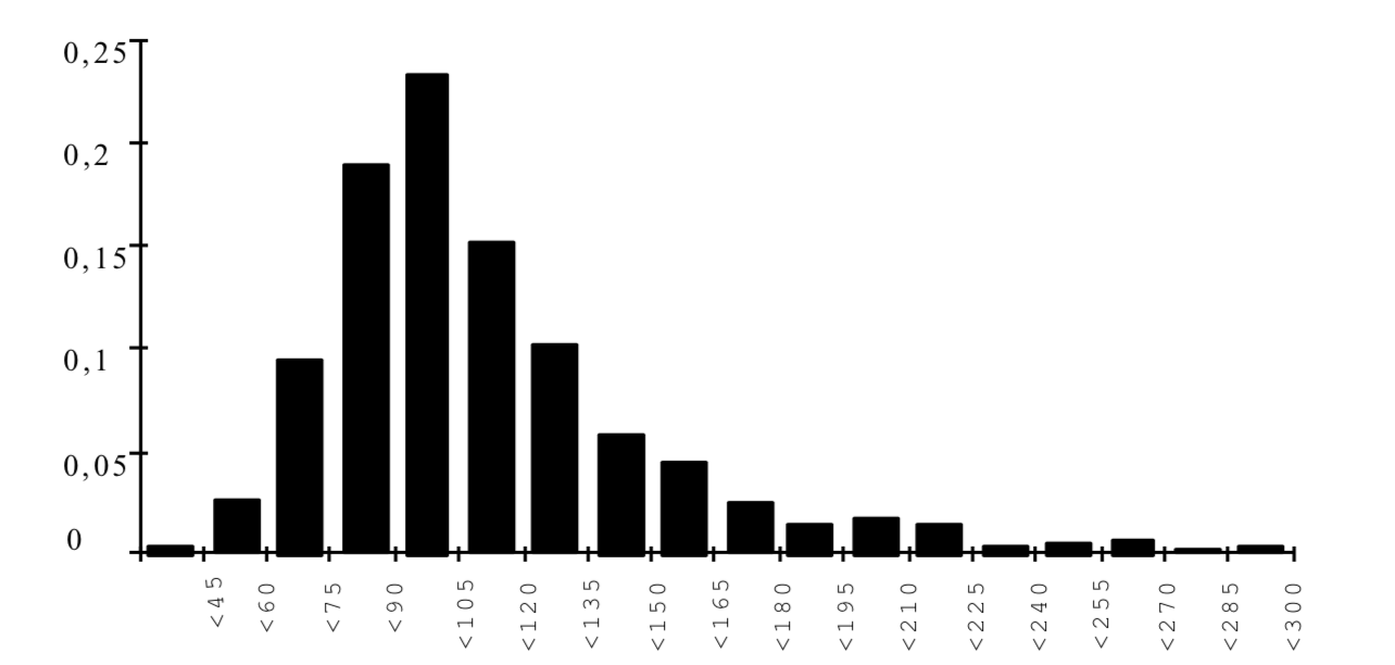
We should say that the obtained index is an abstract index. It does not represent a concrete measurement, centered around 0 and with an arbitrary variance. Using information from other research studies,we can transform the scale of the index in order to have a more conventional scale ranging from 0 to 100. Which provides the following distribution depicted in figure 4.11.

Figure 4.11: Histogram of Economic Capacity Index