3.10 PCA as an Intermediate Analytical Stage

Working with the first principal components provides a handful of advantages: 1) the principal components are orthogonal; 2) the random variability part is minimized; 3) the components provide an optimal dimensionality reduction; and 4) calculating the distances between individuals is simplified.

Often, a problem involves modeling a certain response variable \(\mathbf{y}\), in term of a series of explanatory variables. When the response variable is a quantitative variable we talk about regression models. In turn, we talk about classification when the response variables is of categorical nature.

One common issue when modeling a response variable—with a regression or classfication technique—has to do with multicollinearity in the explanatory variables. Geometrically, the subspace spanned by the explanatory variables is unstable. This means that small variations in the values of the variables will result in large changes on the spanned subspace.

Performing a regression analysis involves projecting the response variable onto the subspace spanned by the explanatory variables. If two explanatory variables are highly correlated, small variations in these variables will substantially modify the orientation of the space. And consequently, the projection \(\hat{\mathbf{y}}\) becomes unstable (see figure 3.8)

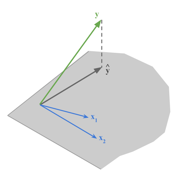
Figure 3.8: Orthogonal projection of y onto the plane spanned by two explanatory variables x

In this situation, and with more than two variables, it can be interesting to use the principal components obtained on the data table \(\mathbf{X}\) formed by the explanatory variables. More specifically, we can keep those components for which their eigenvalues are sufficiently different from zero.

Because the principal components are expressed as linear combinations of the explanatory variables, we can use the components to define the projection subspace for the response variable.

By using only the first principal components, we reduce the random variability in the data. Therefore we can say that the data have been “smoothed”.

One is left with the operation to undo the change given by using the components. That is, we need to express the response variable in terms of the original variables. Each principal component is written as a linear combination of the explanatory variables:

\[ \mathbf{y} = b_0 + b_1 \Psi_1 + \dots + b_p \Psi_p = \hat{\beta}_0 + \hat{\beta}_1 \mathbf{x_1} + \dots + \hat{\beta}_p \mathbf{x_p} \tag{3.9} \]

The principal components in this case become instrumental variables. This means that they behave like intemediate links for a another subsequent analysis.

We can select the principal components that will be part of a given model. One way to do this is by selecting them with the Furnival-Wilson (1974) algorithm to obtain the best regression equations. In fact, the problem is much simpler given that the factors are orthogonal.

An analogous situation occurs within a classification context. As a particular case, the discriminant analysis of two groups is equivalent to a regression analysis. In this case, we can have a preliminary selection of those principal components with the most discriminant power.