3.6 Synthetic Variables and Indices
So far we have discussed Principal Component Analysis from a purely geometric perspective: how to obtain a subspace that best approximates the original distances of the data elements.
Interestingly, PCA can also be approached from other points of views. One of them involves looking for a small set of new variables—formed by the original ones—in such a way that the loss of “information” is minimized.
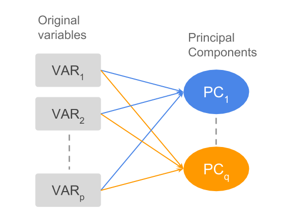
Figure 3.3: Dimension reduction or minimization of “information loss”
The new variables (i.e. vectors) are searched for in a way that they are as close as possible (as much correlated as possible) to the set of original variables. We can think of these new variables as synthetic variables.
The solution is obtained with the vector \(\Psi\) of \(n\) elements that maximizes the function (3.7)
\[ \max \sum_{j} cor^{2} (\boldsymbol{\Psi}, \mathbf{x_j}) \tag{3.7} \]
In other words, we look for a new variable that is the “closest” to the set of original variables. This will provide a first common factor; the rest of the factors are obtained with the same condition but orthogonal to the directions previously obtained.
Often, the first factor is highly correlated with all the variables. This indicates the so-called size factor, which we have discussed in detail in section 2.3.
The size factor can be considered as an overall summary, or synthesis, of the entire set of variables. We can compare the first factor with the average of all the original variables, and notice that they are very similar.
\[ \frac{1}{p} (\mathbf{x_1} + \mathbf{x_2} + \dots + \mathbf{x_p}) \approx \boldsymbol{\Psi_1} \tag{3.8} \]
| Variable | Coord1 | Coeff1 |
|---|---|---|
| teacher | 0.94 | 0.30 |
| bus_driver | 0.96 | 0.30 |
| mechanic | 0.92 | 0.29 |
| construction_worker | 0.90 | 0.28 |
| metalworker | 0.95 | 0.30 |
| cook_chef | 0.87 | 0.27 |
| factory_manager | 0.84 | 0.26 |
| engineer | 0.90 | 0.28 |
| bank_clerk | 0.88 | 0.28 |
| executive_secretary | 0.97 | 0.31 |
| salesperson | 0.96 | 0.30 |
| textile_worker | 0.94 | 0.29 |
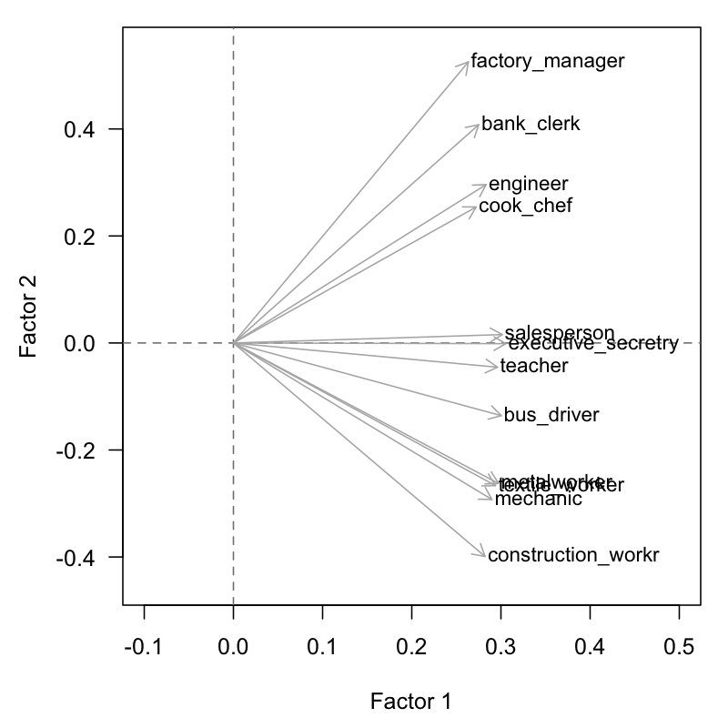
Figure 3.4: Size Factor of active variables
The data set about the international cities provide an example of how to find an index of mean salary per city. The components of the unit axis give the linear combination of the original variables (mean-centered and reduced). This is the linear combination of the first principal component, namely, the desired index of mean salaries (see table 2.3).
A common application of PCA is to build synthetic indices. For instance, a quality index of a given product made from several characteristics of the product. A common example in psychometrics has to do with indices that define a general aptitude factor: e.g. verbal aptitude, or math aptitude. Also in economics, we often find indices of economic capacity for a certain region or city.
Sometimes there is no clear definition of the desired index, but rather a vague notion of the aspects that such an index may comprise. In these cases, the analyst must pay careful attention to collect reliable data, with indicators of the desired index, ideally with highly correlated variables. The computed index (or a first approximation) will be determined by the first principal component of the gathered data.